
feature
Modeling the Coronavirus Outbreak for Cross-Discipline Teaching
Journal of College Science Teaching—November/December 2020 (Volume 50, Issue 2)
By Joseph J. Molitoris
The Coronavirus outbreak allows for a number of possible applications to classroom teaching (biology, computer science, Earth science, physics, statistics), as well as student research. A number of simple models reproduce fairly well the case numbers (total confirmed cases) of the Coronavirus pandemic in specific regions. These models may also be used to predict future cases and can be updated as data become available in a region (city, state, country).
The Coronavirus outbreak allows for a number of possible applications to classroom teaching (Molitoris, 1992) as well as student research (Molitoris, 2016, 2017). In mathematics or computer science courses, the topic of analytic models and computer modeling is relevant. In biology or Earth science classes, the topic of disease and its impact on population is important. In calculus or physics, we often explore exponential growth and computer models. The professor may use the pandemic as part of a classroom lesson or include the topic as a student research project. I have done both over the years with similar topics (Molitoris, 2016, 2017). If used as part of a group of student research projects, a poster session can be conducted to showcase the projects. Further, the papers can be collected in a bound proceedings collection that is edited by the instructor and published either online or as a paper yearbook.
Models can also be used by decision makers to guide their way through the exigencies of this or other pandemics. Students will be familiar with the governmental use of data and models from the daily and weekly Coronavirus briefings from governors and the White House. Decisions about social distancing, travel restrictions, and the imminent opening of states and countries for normal business are influenced by both actual data and models.
Initially, I tried a simple Poisson model (Olkin et al., 1994), but decided that it does not describe the data well enough (Olkin et al., 1994; CDC, 2020; New Jersey Department of Health, 2020; Raychaudhuri et al., 2020; NYC Health, 2020). This is probably because the Poisson probability distribution p(n) only has one parameter lambda (Olkin et al., 1994).
Thus, I investigated the use of the binomial distribution, which along with a number of trials n, has a parameter p that may be thought of as an infection probability for a susceptible population. If the growth curve of the region being modeled indicates more than one outbreak, then more than one binomial distribution helps to describe the cumulative number of cases. See Figure 1 for a comparison of the World Health Organization China data to the binomial distribution model (WHO, 2020).
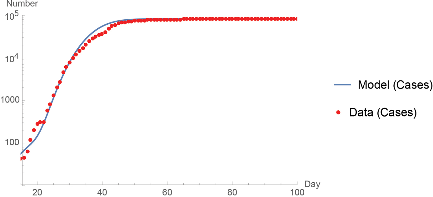
A comparison of the World Health Organization China data (2020) to the binomial distribution model.
Second, I looked at a simple logistic equation model that can describe all or part of the data for a region. A long start-up phase can make it difficult to nonlinearly fit the two parameters S and r. Nevertheless, in many cases this model works very well. See Figure 2 for a comparison of the World Health Organization Germany data to the logistic equation model (WHO, 2020). The correlation coefficient r2 is 0.996.
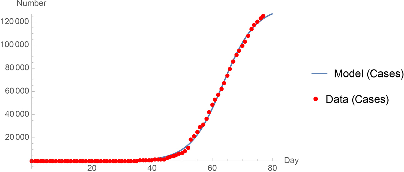
A comparison of the World Health Organization Germany data (2020) to the logistic equation model.
Third, and finally, a basic time stepped simulation (Molitoris, 1992) can be used to describe the data in a region. Again, there are two parameters S and r. S, the “susceptible,” is the long-term population that becomes infected; r is the growth rate or transmission coefficient. The differential equation that the computer simulation solves is: dy/dt = r y (1-y/S). The precision of the simulation can be verified by comparison to both exponential growth and logistic model growth, respectively. With a time step of 0.1 day in the simulation, the percent error versus the logistic equation is typically less than 0.1 %; we use .01 day in the simulations shown here. See Figure 3 for comparison of Centers for Disease Control and Prevention U.S. data during the pivotal month of March 2020 to the time-stepped simulation model (CDC, 2020).
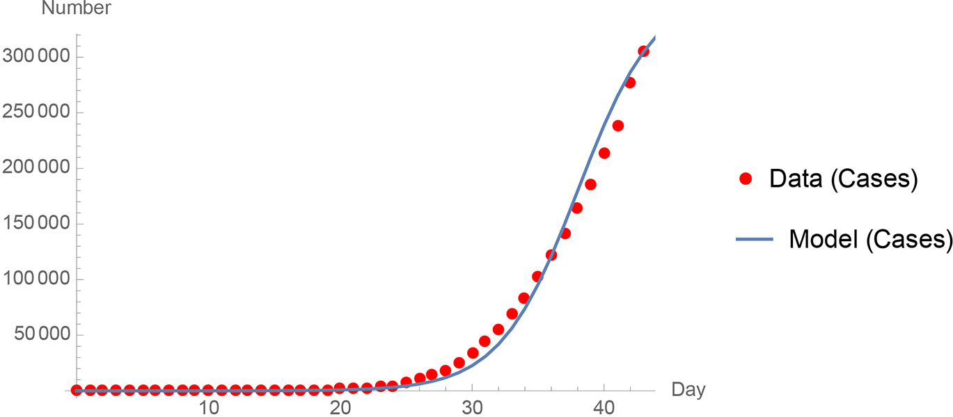
Comparison of Centers for Disease Control and Prevention United States data (2020) during the pivotal month of March 2020 to the time-stepped simulation model.
I have also compared the Coronavirus data for other countries (England, France, South Korea, etc.), select states (NJ, PA, NY), and cities (New York City and Los Angeles) to the three models previously described. In all cases, fairly good representation of the data is seen. The data may be found by student or teacher online either as the pandemic progresses (as an at-home lesson or summer project) or from archived data once the crisis is over (Olkin et al., 1994; CDC, 2020; New Jersey Department of Health, 2020; Raychaudhuri et al., 2021; NYC Health, 2020).
Further work by students can be more sophisticated if desired. The single differential equation is changed to a coupled set of four equations: (1)dy/dt = r y (1-y/S-R/S-D/S) - b y - d y (2)dx/dt = -r y (1-y/S-R/S-D/S) (3)dR/dt = b y (4)dD/dt = d y
where y is the number of infected, × is the number of susceptibles, R is the recovered, and D is the deaths. Note that since × + y + R + D = S, a constant, the sum of the above differential equations is zero. The parameters b, d, r, and S must be extracted from experimental data of the pandemic and can be adapted to the situation as the disease spreads. The initial conditions that permit the solution of the differential equations using a fixed time step procedure are that at t = 0, we have y = 1, R = D = 0, and × = S-1. The basics of this type of modeling were developed over 100 years ago (Kermack & McKendrick, 1927) and are still in use today in a variety of contexts.
See Figure 4 for a comparison of the World Health Organization World data (2020) to my Coronavirus differential equation model (equations 1 through 4 programmed in Mathematica [Wolfram, 1988]). The representation cannot be perfect since early on (January 2020) China drove the world numbers and as of May 2020 the United States and Europe drove the growth. The representation here is pretty good: the correlation coefficient is 0.98 for the cumulative confirmed cases and cumulative deaths.
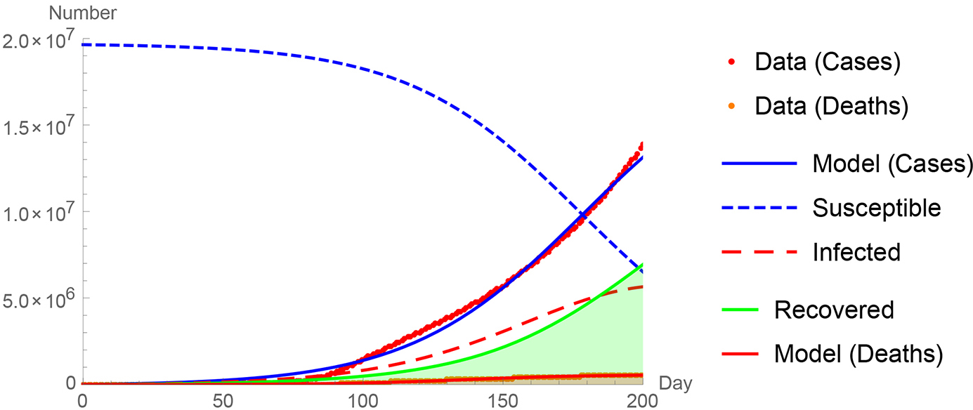
A comparison of the World Health Organization world data (2020) to my Coronavirus differential equation model (equations 1 through 4 programmed in Mathematica).
Finally, I want to point out that both noise and harmonics (which are present in the data) can be easily added to the differential equation model (Molitoris, 2020). If this is done, then one can do a fairly good job of reproducing the orbits of the Coronavirus evolution in most regions. The result is shown in Figure 5 for the state of New Jersey in the United States. The orbits come from simply plotting the new deaths versus the new cases as opposed to the cumulative numbers, which are more commonly seen. In Figure 5, each orbit is counterclockwise as the cases and deaths first increase, reach a maximum, and then decrease to mathematical extinction as the pandemic dies out in a region.
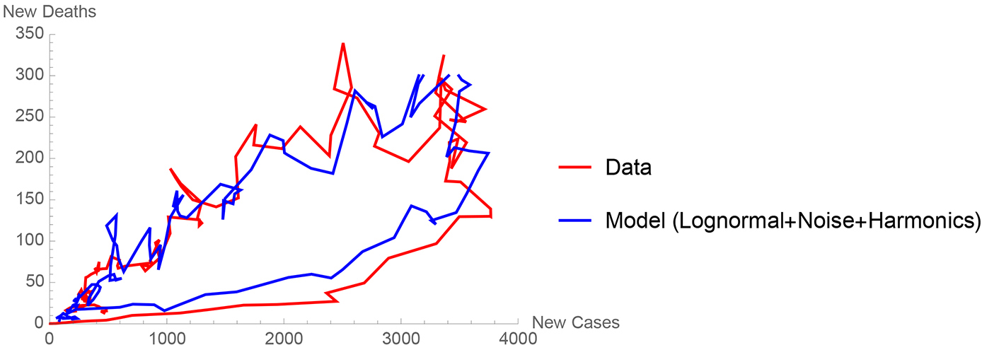
A comparison of the Center for Disease Control New Jersey data (New Jersey Department of Health, 2020) to my Coronavirus differential equation model (equations 1 through 4 programmed in Mathematica) with the addition
In conclusion, the Coronavirus outbreak allows for several possible modeling approaches. A number of simple models reproduce fairly well the case numbers (total confirmed cases) of the Coronavirus pandemic in specific regions. An extended model that includes recovery and death also reproduces the death case numbers. These models may further be used to predict future cases and updated as data become available in a region (city, state, country). Because the models are not complicated, they can be used by decision makers to guide their way through the exigencies of this or other pandemics. I have run the models on a personal computer with Excel and a MacBook Pro with Numbers and Mathematica applications (Wolfram, 1988).