
feature
Walking the Slope
A graph underfoot

CONTENT AREA Physical Science
GRADE LEVEL 6–8
BIG IDEA/UNIT Graphing in motion analysis
ESSENTIAL PRE-EXISTING KNOWLEDGE Some understanding of speed and velocity, as well as basic graphing skills
TIME REQUIRED One class period
COST $10 for tagging tape of two colors, although any string or similar material can be used
SAFETY Students should wash hands after activity.
Tired of your classroom’s worn-out linoleum floor? Wait! Don’t tear it up yet. Look down with an appreciative rather than critical eye. Those gritty squares form the perfect grid for a person-sized graph, big enough for students to physically walk “rise over run” to develop an understanding of slope, taking advantage of middle schoolers’ energy in a kinesthetic learning exercise.
Graphing is key to data analysis of lab concepts in my physical science class: time versus temperature, identification of phase changes, density determination with line of best fit, and distance versus time in speed and velocity. Creating and interpreting graphs is a skill practiced throughout the year, and we coordinate our work with math classes for reinforcement. Such work is central to understanding scientific data; NGSS Scientific and Engineering Practices 4 emphasizes that “data must be presented in a form that can reveal patterns and relationships . . . [and] a major practice of scientists is to organize and interpret data through tabulating, graphing, or statistical analysis.” I developed “A Graph Underfoot” for an alternative approach to the understanding of graphs through kinesthetic individual participation and class discussion. Following the activity, the class as a whole expressed significantly increased confidence in their understanding of graphing and slope. An extension to this activity is to have students collect data for a purpose, then walk-graph their own data as a way to understand how their data tables translate to a graph. However, because working with their own data adds complexity as well as anxiety about their results, the goal of this activity was to help students develop very basic graphing skills.
Materials required
- Blue painter’s masking tape
- Sticky notes
- Clear packing tape (useful in putting over sticky notes to keep them in position)
- Plastic survey tape (at least two colors)
Graphing activity
The activity itself is fairly simple. Prior to class, I clear a square approximately 4 × 4 meters of classroom furniture. With simple materials (see callout box) I create the x and y axes along the left and bottom edges with blue painter’s masking tape, marking each line between floor tiles numerically. The result is a 7 × 10 grid of floor tile squares; tile joints form the grid lines of the graph. (Note that this activity could be easily and quickly adapted for nontiled floors by creating the grid with painter’s tape). I then create sticky notes with the important labeling components of a graph but do not place them (see Figure 1). As this particular example comes from introductory motion physics, the x- and y-axis measurements were time (in seconds) and distance (in meters).
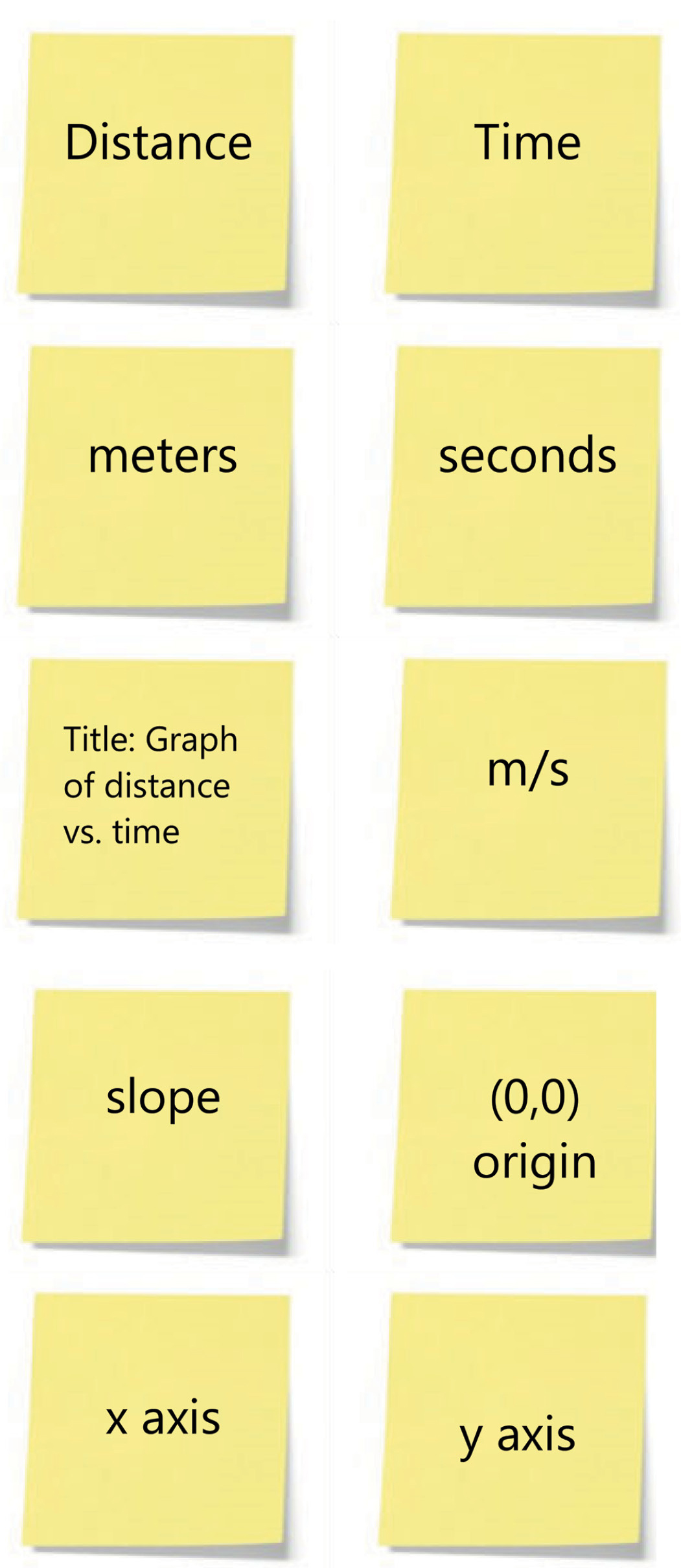
Sticky note labels for “Graph Underfoot.”
The activity begins with a pretest that emphasized understanding of the units and measurements used in calculation of speed and velocity (see Online Supplemental Materials). After a short discussion of the answers, the class gathers around the outside edges of the graph area. I introduce the area as a graph and ask the students what important components of a graph were missing; as they suggest labels, units, title, and so forth, I produce the labels for them to place in the correct locations. An alternative approach would be to have the students create the labels themselves during the discussion. Students’ attention and interest is maintained by making them active participants in creating the group graph, answering questions such as: Who has the “title” sticky note? Where should it be placed? (Note: there are many possible stickies; I suggest teachers make up as many as they need, and try to make sure that each student participates in at least one sticky note placement).
Once we agree that the graph components are complete we begin to plot data points (see Figure 2). One end of a roll of survey tape is taped to the origin (0,0) of the graph. Individual students, with the help of their classmates, then place the survey tape on the graph to represent motion that I describe. The motion scenarios are as follows:
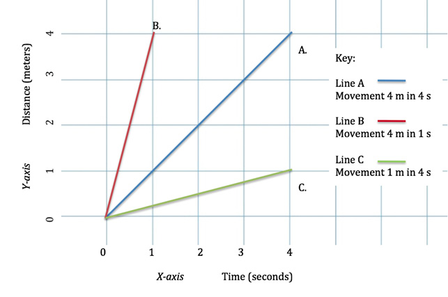
Graph of activity scenarios A, B, and C.
- Scenario A: The student starts at the origin (0,0) and walks 4 meters in 4 seconds. Graphing procedure: After the survey tape is fixed to the 0,0 location with the painter’s tape, I direct the student to walk first the rise (4 meters), then to turn a right angle and walk the run (4 seconds), taping the other end of the survey tape at the end coordinates (4,4). The student then breaks off the rest of the roll of survey tape. Students can see that the end point (4,4) is determined by both the x and y coordinate values and can immediately see how the slope is generated by this motion.
- Scenario B: The student starts at the origin (0,0) and walks 1 meters in 1 second.
- Scenario C: The student starts at the origin (0,0) and walks 1 meter in 4 seconds.
Student focus can be maintained by emphasizing that the task is for completion as a group. I choose a different student for each scenario and check in with the class as a whole for comments, corrections, and questions as each graph is created. Once students are comfortable with these relatively simple graphs, I introduce more complex “extension” scenarios to help them understand the relationship between change in slope with change in motion (see Figure 3). Note that each change in motion will require students to tape the surveyor’s tape in place before the change in slope.
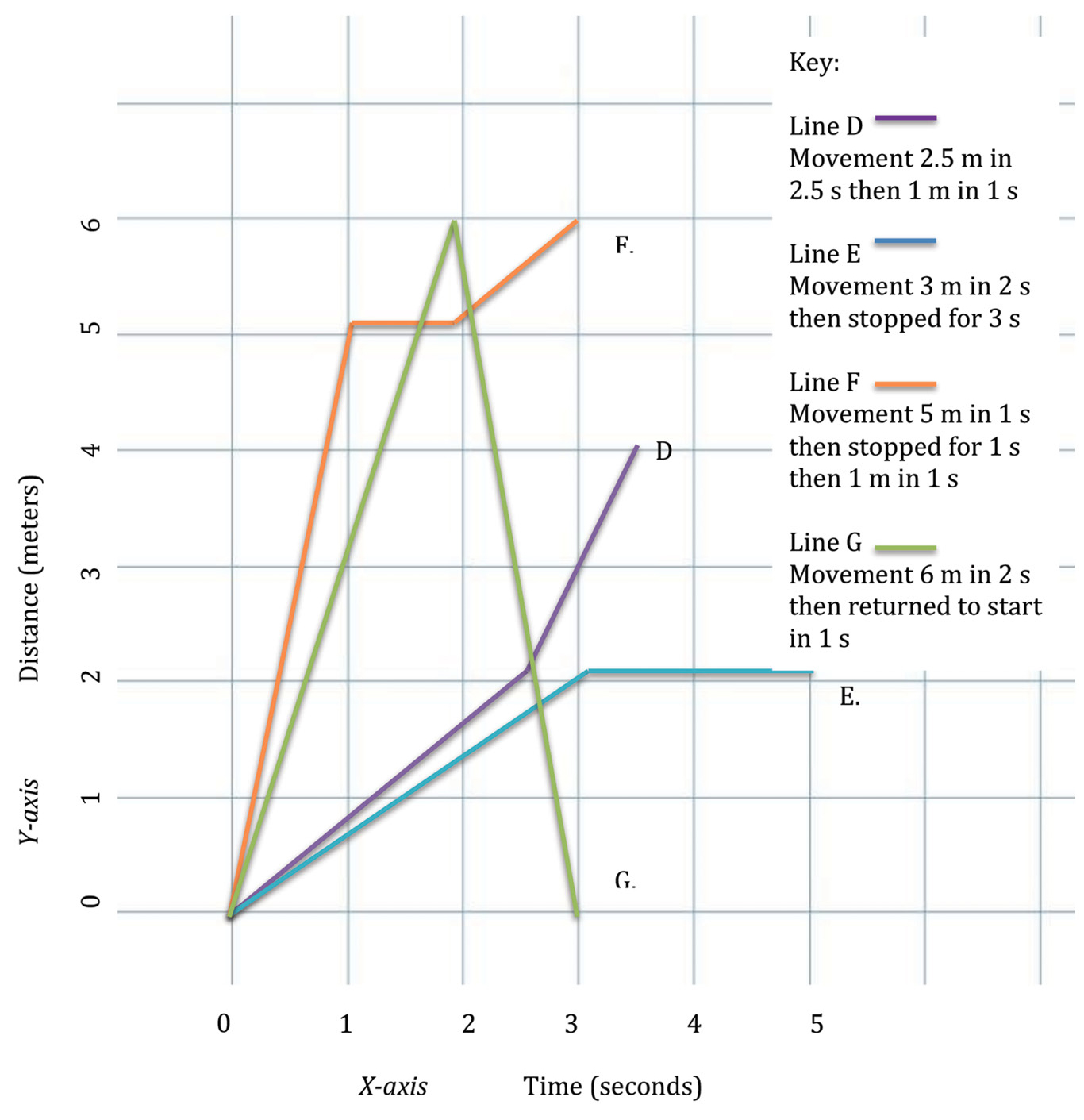
Graph of activity scenarios D, E, F, and G.
- Scenario D: The student starts at the origin (0,0) and walks 2.5 meters in 2.5 seconds, then walks 1 meters in 1 seconds.
- Scenario E: The student starts at the origin (0,0) and walks 3 meters in 2 seconds, then remains stopped for 2 seconds.
- Scenario F: The student starts at the origin (0,0) and walks 5 meters in 1 second, stops for 1 second, then continues for 1 meter in 1 second.
- Scenario G: The student starts at the origin (0,0) and walks 6 meters in 2 seconds, then returns to the original starting location in 1 second.
Coordinates of the motion scenarios A through C are chosen to demonstrate contrasting relationships between slope and speed (differing slopes represent different speeds). I carefully lead the students through a discussion of how slope reflects speed: the steeper the slope, the faster the speed. Scenarios D through G introduce the concept that change in slope represents change in speed and/or direction (velocity). Each of these scenarios is designed to introduce an important concept in graphing motion. Scenario D introduces the connection between change in slope and change in speed, emphasizing that slope itself is a direct representation of speed. Scenario E and F show that a flat slope represents no movement. Finally, Scenario G introduces the idea of negative slope as motion in the opposite direction. This scenario is particularly challenging to students—in many cases they want to bring the line back to the origin. After discussion, they realize that they cannot go backward in time, but they can in space, and create the correct graph.
After each scenario, I ask the class to determine the line’s slope or slopes (see Figure 4). Following this, discussion emphasizes the use of “rise over run” for the determination of slope. Students notice that the graph can be read like an equation—the y-axis coordinate over the x coordinate, with the graphed line itself forming the line separating numerator from the denominator. As students walk the coordinates, they immediately see the direct correlation between change in motion and change in slope. Each slope remains on the graph throughout the activity for easy comparison and discussion. This activity compliments the Science Sampler “Walk This Way” (Fechheim and Nelson 2007), which offers challenging extensions to the basic graph development outlined here.
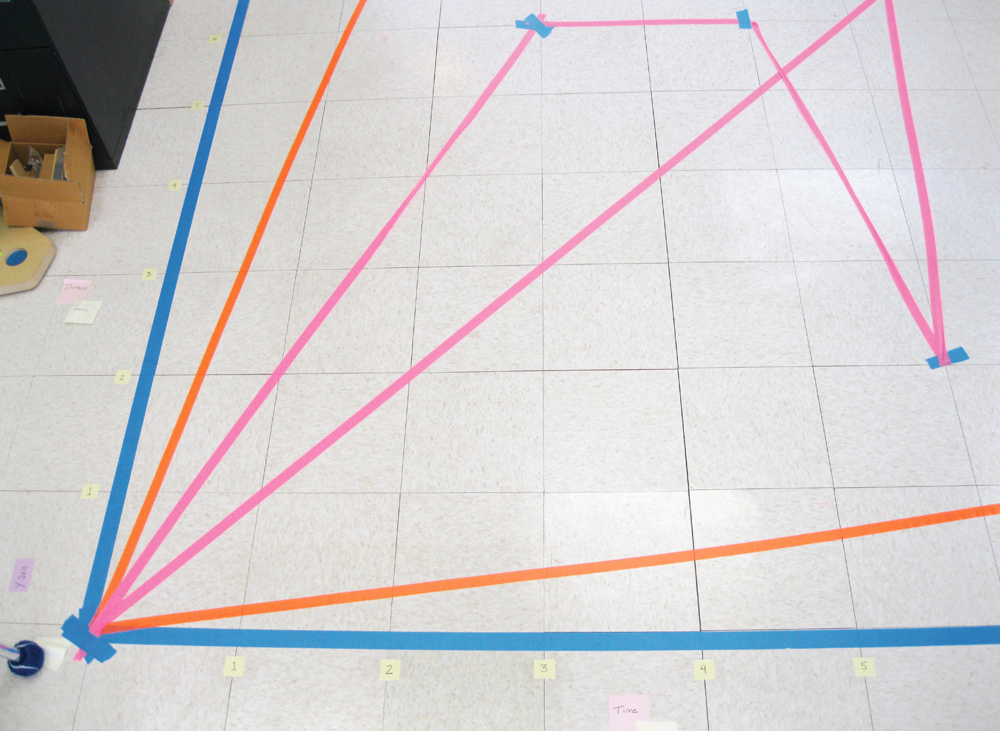
Graph under construction on classroom floor.
Conclusion
Physically walking the speeds or velocities allows students to immediately see the resulting changes in slope. Furthermore, the direct physical translation of data into graph outlined in this activity can be especially helpful for students with learning difficulties, students who are visual learners, and students who struggle with language (English language learners). These learners are also helped by the deliberate stepwise fashion through which each scenario is developed and graphed, modeling the thought processes that will be needed for them to complete similar challenges on their own. Significant improvement is seen on the postactivity assessment (see Online Supplemental Materials). Students respond very positively to this exercise—“oh . . . I finally get slope!” exclaimed one 8th grader on completing the activity. •
ONLINE SUPPLEMENTAL MATERIALS
Preactivity assessment—https://www.nsta.org/online-connections-science-scope
Postactivity assessment—https://www.nsta.org/online-connections-science-scope
Catherine E. Hibbitt (chibbitt@lincolnschool.org) is a middle and upper school science teacher at the Lincoln School in Providence, Rhode Island.
Physical Science Teaching Strategies Middle School