It’s true that being in the right place at the right time can lead to new scientific discoveries. Velcro, Corn Flakes, super glue, the Big Bang, and Brownian motion were all discovered serendipitously. Nevertheless, being in the right place at the right time is not sufficient. Discovering new phenomena requires curiosity, creative thinking, and the right tools.

In 1827, Robert Brown noticed pollen suspended in water bouncing around erratically. It wasn’t until 1905 that Albert Einstein provided an acceptable explanation of the phenomenon (Kac 1947): Brownian motion is the random movement of particles (e.g., pollen) in a fluid (liquid or gas) as a result of collisions with atoms and molecules. Movement of the particles is random. Atoms and molecules move and collide with particles as a consequence of thermal energy defined by temperature.

The activities described in this paper address NGSS HS-PS3-2 (see NGSS chart, page 51). Brownian motion provides direct evidence of molecular motion, and can be directly observed. However, because it is not possible to track the movement of every atom or molecule, probability models can be used to effectively illustrate particle movement.

The thermal energy of Brownian motion is necessary to explain the random movement of particles from a high to low concentration (Weiss 2017), the spontaneous movement of a solvent through a membrane (Odom, Barrow, and Romine 2017), the particulate nature of liquids and gases (Wiseman 1979), and movement of particles (such as proteins) within cells. Brownian motion in an unbound environment (Bressloff 2014) causes particles to randomly move in multiple directions. The surrounding thermal energy supplied to atoms and molecules causes the movement.

Metabolic energy of a cell does not directly cause movement (e.g., particles in and out of a cell); the movement is caused by Brownian rectification. Cell energy is used to rectify Brownian motion by establishing boundary conditions. Metabolic energy triggers the establishment boundary conditions via protein secondary, tertiary, and quaternary structures. Metabolic energy does not directly cause movement; rather, the mechanical energy conversion is caused purely by the thermal energy of Brownian motion, resulting in the one-way movement of particles (Fox 1998).

Models of Brownian motion have been documented over the past four decades. Knapp (1980) described constructing a model of molecular motion using marbles and a box. Kruglak (1989, 1994) reported using television technology to project the image of a drop of white glue with water to allow the whole class to view molecular motion. He also found that projecting a laser beam into a mixture of water with sage, mace, thyme, apple pie spice, mustard seed, or ginger allowed the class to observe molecular movement. Schultz (1990) accidently discovered that a 1-milliwat helium-neon laser beamed through a suspension of starch could be used to project molecular motion on the wall of his classroom.

This paper provides a theoretical framework with four associated laboratory activities (Appendix A, Labs 1 through 4) designed to guide construction of knowledge about Brownian motion. Lab 1 involves the direct observation of Brownian motion with a microscope and cell phone camera. Lab 2 guides students to make hypotheses and construct tentative models of random movement of particles based on the experience of a random walk. Lab 3, facilitated by computer technology and Excel software (see “On the web”), provides opportunities for comparisons of multiple models of a random walk, and Lab 4 concludes the instructional sequence with the use of an interactive model of Brownian motion.

Understanding of Brownian motion can be developed as both declarative and procedural knowledge. Declarative knowledge refers to “knowing the answer to” and procedural refers to “knowing how to” (Gagne 1985). Each knowledge type has corresponding question types that best elicit that knowledge from students.

Declarative knowledge questions ask for recall of specific information. Learning strictly through textbooks, lectures, and memorization, independent of directly observing and experiencing phenomena, often produces limited declarative knowledge. It does not lead to the conceptual understanding valued for scientific literacy. However, declarative knowledge gained through observations, experiences, and engagement in the scientific process can lead to conceptual understanding.

Procedural knowledge questions ask for sense-making. Procedural knowledge is associated with two question types: (a) descriptive questions, which can be used to identify or describe interesting phenomena, and (b) causal questions, which can be used to ask why a phenomenon occurs. Asking why a phenomenon occurs promotes construction of hypotheses to provide tentative explanations. Learning is more complete when procedural knowledge is used to construct declarative knowledge (Lawson 2001).

Many descriptive questions call for information and data collection beyond the offerings of traditional textbooks, and require procedural knowledge for making observations, inferring, designing experiments, controlling variables, collecting and analyzing data, drawing conclusions, and presenting findings. Descriptive questions are excellent for guiding identification and discovery of important scientific phenomena and make good initial research questions. They ask for systematic observations resulting in data-supported conclusions. For example, by guiding students to observe whole milk, which consists of water, fat, protein, and minerals, it is possible for them to observe milkfat droplets moving erratically (Brownian motion).

Of course, it is also possible to look up this phenomenon in a textbook. But, to support engagement in scientific processes for making sense of interesting phenomena, descriptive questions guide systematic observations.

Constructivist and sociocultural views of learning frame the laboratory activities described below. These views of learning posit that knowledge construction occurs through reflective thought (Fosnot 1996) and that social interaction is an essential part of the learning process (Vygotsky 1978). Furthermore, a range of knowledge that might be out of reach for an individual student may be accessible with support from peers and “more knowledgeable others” (Vygotsky 1978).

These labs are particularly well-suited to the construction of knowledge with diverse student populations because they are experiential, guided by “a more knowledgeable other,” and encourage reflective thought. Students engage both physically and socially—they have direct experiences with scientific phenomena and engage in scientific discourse informed by the experiences. Visual and physical experiences along with scientific discourse lead to opportunities for formulating explanations and hypotheses, developing and using models, and engaging in argumentation.

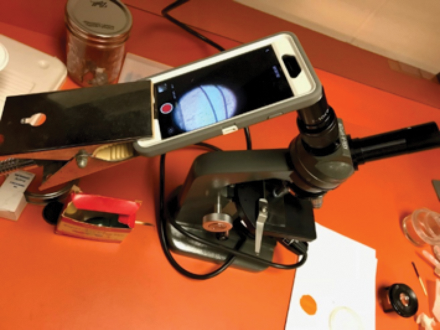
Lab 1 initiates knowledge construction about Brownian motion as students observe the movement of milkfat droplets (Figure 1). This lab provides an opportunity to experience and think about a physical phenomenon before working with a model. The following questions and prompts are used to guide observations:

• What do you see when whole milk is examined under a microscope? Possible observation: The milk (fat) is bouncing around under the slide.
• Can you see what is causing the milk to bounce around? Have you seen similar phenomena? Describe the motion you see. Possible observation: Answers will vary. It is not possible to see what is causing the motion. Students can share ideas and/or explanations and argue, based on observational and experiential knowledge, which ideas or explanations best represent the phenomenon.

Experimental design is not limited to laboratory conditions. Some scientists use thought experiments based on scientific laws and embedded theories. Thought experiments play an important role in scientific inquiry (Gendler 1998) and have been used to explain molecular motion. For example, Maxwell’s Demon was created by James Clerk Maxwell in 1867. His experiment suggested that fast and slow molecules moving into a chamber could potentially violate the second law of thermodynamics. Additionally, Einstein advanced a thought experiment to explain Brownian motion as a free particle being struck by molecules as described by probability density.

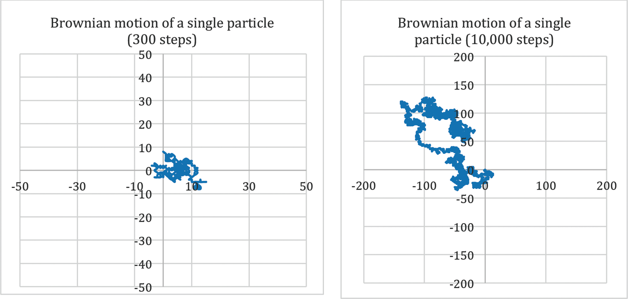
Labs 2 and 3 are thought experiments enhanced by activities to explore movement of a free particle as described by Einstein. During Lab 2, students physically take a random walk using coin flips to determine their walking direction and record the path of the walk (Figure 3). If students compare their random walk to the results of other groups in the class, they will find that theirs is completely different. Subsequently, in Lab 3, an Excel spreadsheet is used to simulate random walks repeatedly, using Excel functions to randomly generate the 0s and 1s that determine the path (see Figure 3 as an example). On the left side of Figure 3, a 300-step random walk representing Brownian motion is shown. On the right, a 10,000-step random walk is shown.

The following questions guide the thought experiments:

• How does the diagram of a random walk compare to the motion of fat particles in Lab 1? Possible response: Like the random walk, the milkfat droplets in Lab 1 moved around randomly. For the random walk, the direction was determined by chance (a flip of a coin).
• How does the graphed data of simulated walks in Excel, one with 300 steps and one with 10,000 steps, compare to Labs 1 and 2? Possible response: If the line represented the movement of a particle, the particle appeared to be moving erratically in both cases.

Scientific modeling is an important tool for helping students understand, define, quantify, visualize, or simulate scientific phenomena based on evidence and reasoning (Treagust et al. 2002), and has received great emphasis in the NGSS scientific and engineering practices and crosscutting concepts (NGSS Lead States 2013). Pattern recognition and proposing, revising, or defending explanatory models can occur after or concurrently with data collection and analysis. Models may include drawings, diagrams, computers, mathematical derivations, and prose.

Using the evidence gathered in Labs 1, 2, and 3, students are asked to begin to formulate a possible explanation of Brownian motion. For example, students have observed fat droplets in milk under a microscope and noticed that the droplets seem to bounce around erratically. It is not possible to see what is causing the erratic movement of the droplets, so when observation evidence from Lab 1 is combined with information from the random walk experience and simulation (Labs 2 and 3), students have adequate data for developing a plausible model of particle movement.

Formulating hypotheses is perhaps the most important activity associated with exploration of causal phenomena. Providing plausible explanations of phenomena is a high point of critical thinking and problem solving, and should be a major goal of science instruction. However, development of this skill can be challenging. Exploration guided by descriptive questions may facilitate students’ formulation of a causal question. Hypotheses are constructed to explain the phenomenon, experiments are designed and conducted to test hypotheses, expected outcomes are determined, and conclusions are drawn. It should be emphasized to students that hypotheses are not “best guesses” but plausible explanations based on prior knowledge, logic, and observations.

Conclusions drawn from models developed to investigate newly formed hypotheses should always be considered tentative. Students should be encouraged to consider variables that were not controlled, potential confounding variables, and potential errors that may have occurred during model construction. Additional research may be necessary to support or refute tentative hypotheses—the process of scientific inquiry is never-ending and the results are never final.

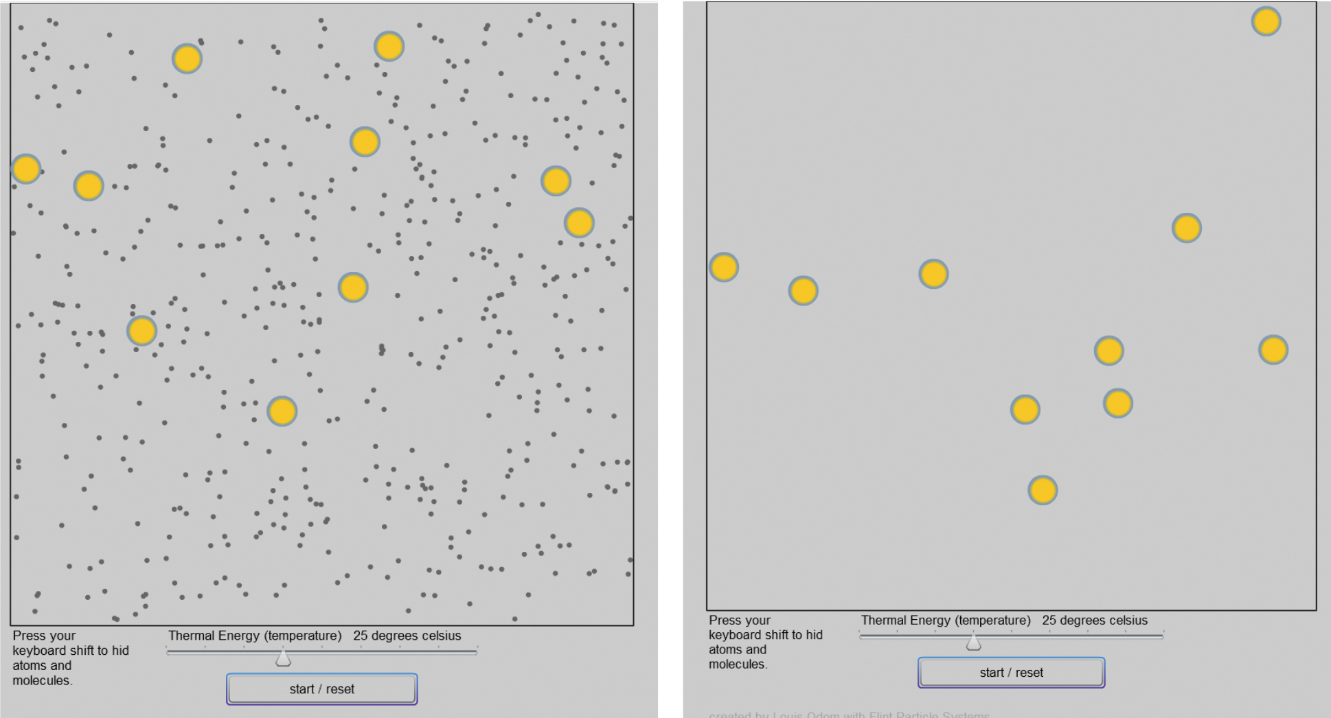
Lab 4 provides a computer model to illustrate small particles (atoms and molecules) moving around and striking larger particles (milkfat droplets, which then appear to be moving randomly), a possible cause of Brownian motion. The computer model allows the user to hide the atoms and molecules to compare the larger particle movements to a random walk. Thermal energy can be adjusted to change the speed of the particles. The following descriptive questions guide Lab 4.

• Describe Brownian motion using evidence from each previous lab to describe the phenomena. Possible responses: In Lab 1, we were able to observe the movement of milkfat droplets. The initial random walk (Lab 2) illustrated the movement of a single particle, which might be related to what we saw in Lab 1. The chance of moving right, left, forward, and backward with each step was equal. With Lab 3, in Excel, we created of models of random walks with hundreds or thousands of steps. The Excel model could be run repeatedly. The repetitions confirmed the random movement.
• How might the computer model (Lab 4) be used to represent Brownian motion? Possible responses: We saw fat droplets moving around erratically (by colliding with atoms and molecules, e.g., water) that were not visible in the milk (Lab 1). The computer model showed random movement of particles, which resulted from atoms and molecules striking the particles. When the atoms and molecules within the computer model were hidden, the view of Brownian motion resembled what we saw in Lab 1.

Note to teachers: Discussion of prior experiences before beginning the lab sequence with at least one of these concepts would add to the value of the experience. For example, discuss the phenomenon of an odor traveling across a room. When a bottle of perfume is opened, over time, one can smell the perfume. What causes the perfume molecules to move from the bottle to your nose? Diffusion. What causes diffusion? Brownian motion supports explanations of diffusion, osmosis, and particle movement.

Materials

• Microscope (at least 100x magnification)
• Slides with cover slips
• Whole milk
• Yellow food coloring
• Cell phone with a video camera

Procedure

In order to observe Brownian motion, a wet mount is prepared to suspend milk in water with a cover slip.

1. Obtain a clean slide with cover slip.
2. Add a drop of milk into the center of the slide.
3. Absorb a small amount of yellow dye with a toothpick and place it in the milk.
4. Add the cover slip.
5. Place the slide on a microscope platform at the lowest level. Focus in on the slide.
6. Continue to increase the magnification incrementally until you reach the maximum magnification of the microscope.
7. Place a cell phone camera near the eyepiece (see Figure 1). Set the cell phone camera to record video.
8. Increase the magnification of the cell phone to the maximum while maintaining focus.
9. Record video for about 10 seconds.
10. Examine the video. Describe your observations.

Question 1: What do you see when whole milk is examined under a microscope?

Question 2: Can you see what is causing the milk fat to bounce around?

Note: To observe Brownian motion, a minimum magnification 400x is required. For the directions above, an iPhone 6 video camera was used to increase the 100x microscope magnification by a factor of 4.

For further exploration of this phenomenon, view a YouTube video of a wet mount slide of milk with a yellow food coloring (www.youtube.com/watch?v=3-7bztD3aRw). The first part of the YouTube video provides an approximate total magnification of 400x using a microscope with a 10x eye piece, 10x objective, and iPhone 6s video camera. The second part provides an approximate total magnification of 1600x using a microscope with a 10x eye piece, 40x objective, and iPhone 6s video camera.

Note to teachers: This lab is designed to mimic the movement of a single milkfat droplet. Before beginning, students need to be reminded to record data and to select an open area for the walk. Small spaces will limit movement.

Materials

• Two coins
• Floor with tiles (preferable)
• Paper to record movement

Procedure

1. Prepare to go on a random walk in small student work groups.
2. Within groups of 2 to 3 students, (no groups of 4), assign a walker, a coin flipper, and a recorder.
3. Students will use a coin to determine the direction of each step. Decide what heads and tails represent (Forward/Backward, Left/Right).
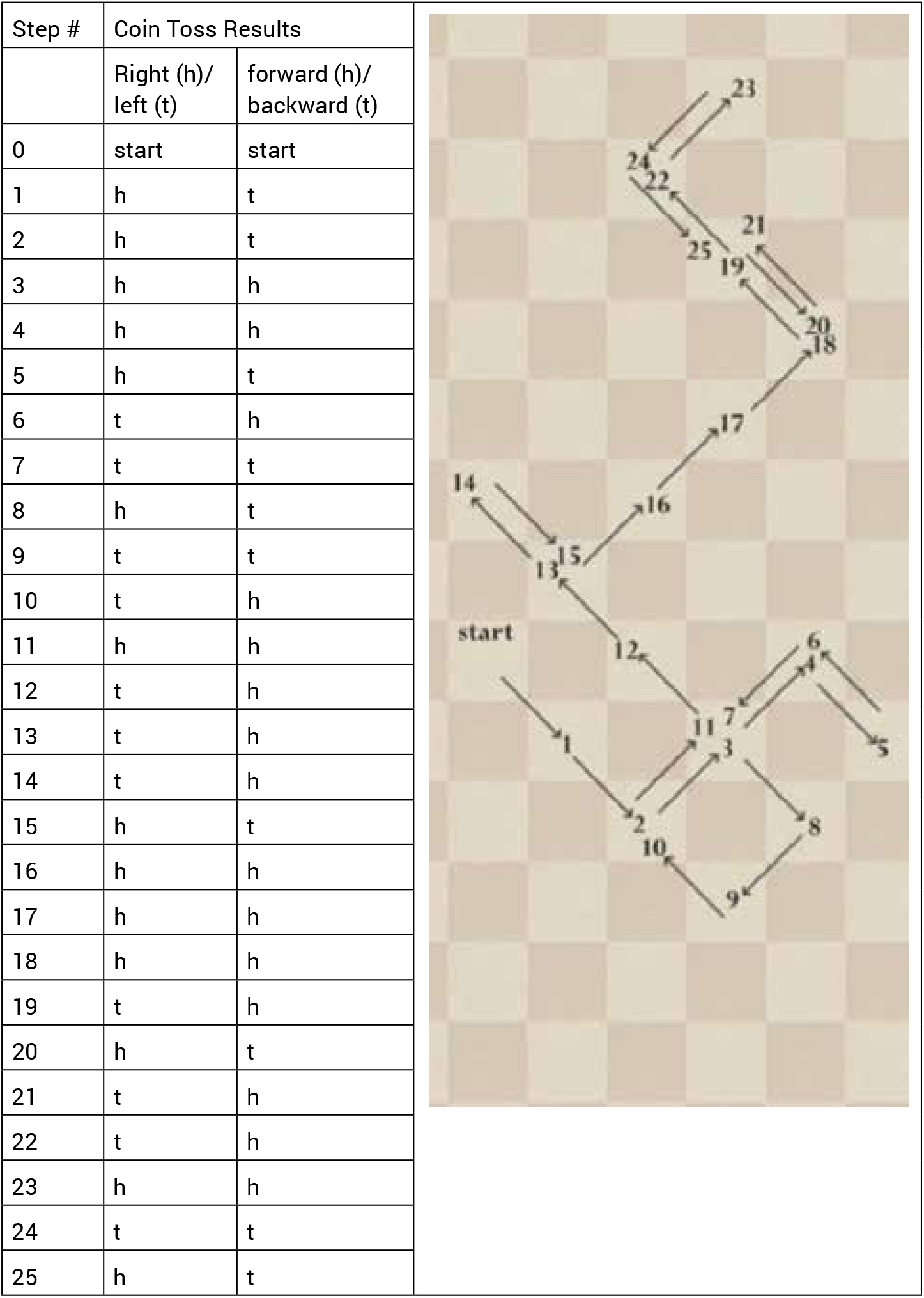
4. Flip the coin twice, once to determine forward/backward and then again to determine left/right. In other words, for each step of the walk, the walker will move forward or backward and left or right (See <a class="fig" href="#TST_43_F2">Figure 2</a>, with example coin flip pairs and a record of a 25-step walk, below). Each coin toss pair is the result of flipping a coin twice to determine a step right or left and forward or backward. In this case, on the first flip, heads=right, tails=left; and on the second flip, heads=forward, tails=backward.
5. Walk at least 25 steps.
6. Record your walk on centimeter grid paper. Compare your diagram to another group’s diagram.
7. Question: How could a random walk be used to represent Brownian motion?

Note to teachers: This lab is designed to mimic the movement of a single milk droplet with technology. Walking 300 or 10,000 steps is not realistic. The spreadsheet allowed students to do the random walk many times.

Materials

• Computer
• RandomWalk.xlsx spreadsheet (available at http://php2.umkc.edu/education/alodom/Science_Teacher/RandomWalk.xlsx)

Procedure

1. Open the Random Walk Excel spreadsheet.
   1. Optional: Choose the Walk-data tab and enter your random walk data to graph your walk.
2. Go to the Brownian motion tab (see Figure 3).
3. At the top of the page, go to Formulas. Find the Calculate Now button on the right side.
4. Select the Calculate Now button.
5. Records observations of the 300 step and 10,000 steps random walk models by printing the screen or using a snipping tool.
6. Repeat selection of the Calculate Now button. Record observations with a snipping tool or print screen.
7. Describe your findings.

Note to teachers: An interesting way to introduce the model is to ask students to draw a picture of Brownian motion of several particles. It’s very difficult to do. Then challenge them to be skeptical about the model after observations and data collection.

Is the model a good representation of Brownian motion? How could it be improved? You could end the lab session with asking students how perfume molecules travel across the room.

Materials

• Computer with Flash player
• Flash movie (available for download at http://php2.umkc.edu/education/alodom/Science_Teacher/brownianmotionmodel3.swf and for viewing at http://php2.umkc.edu/education/alodom/Science_Teacher/brownianmotion.html)

Procedure

1. Open the Flash movie. Select the “start/reset” button (see Figure 4)
2. Record your observations.
   1. Possible observation: Small particles are moving around striking larger particles.
3. Make sure your cursor in over the Flash movie. Select the shift button on your keyboard.
   1. Record your observations.
   2. Possible observation: The small particles are no longer visible but the larger particles continue to move in the same manner, appearing to move erratically.
4. Follow a single particle with the atoms and molecules hidden. Compare the movements of a single particle to the movements from a random walk.
   1. Possible comparison: The larger particle moves and changes direction erratically, similar to a person’s movements in a random walk (Labs 2 and 3).
5. Examine qualitatively the effects of thermal energy on the movement of atoms, molecules, and milk fat droplets. (The user must use the reset button before changing the temperature, and then restart.) 
6. Describe Brownian motion using evidence from each lab to describe and model the phenomena.
7. How could the flash movie model be used to represent Brownian motion?