
start with phenomena
Rainfall, River Height, and Local Relevance
Supporting students’ use of real-world data to explore flash floods
Science and Children—May/June 2023 (Volume 60, Issue 5)
By Lauren E. Brase, Lindsay C. Mossa, and Edward C. Robeck
Floods are among the most frequent and costly natural hazards (CRED and UNDRR 2020), and many locations are experiencing increases in both the frequency and intensity of floods (IPCC 2022). The widespread occurrence of flooding and the fact that both precipitation data and river flow data are readily available for many locations provides an excellent opportunity for educators to bring relevant professionally collected data into their teaching. By connecting those data to the use of models, students can collect, interpret, and communicate about data. In this article we describe a five-day lesson sequence along with design principles that were applied in the lessons. The full set of lessons and supporting materials (slides, handouts, assessments, etc.) are available online (see Online Resources). This curriculum was developed as part of an NSF-funded research project that is being conducted by American Geosciences Institute and the Education Development Center’s Oceans of Data Institute. The lessons are structured to support students’ data literacy skills, conceptual development, and evidence-based reasoning using professionally collected Earth science data. We used data and images from the United States Geological Survey (USGS), Weather Underground, ArcGIS, and Google Earth throughout the lesson sequence.
Ellicott City, Maryland experienced floods in both 2016 and 2018, each of which was considered a 1000-year flood—a potentially misleading term that indicates a flood magnitude that has a .1% chance of occurring in any year. We chose the 2018 Ellicott City flood as our anchoring phenomenon because of its geographic relevance to the students in the 11 classrooms with which we worked in early 2022, though these lessons can be used worldwide as they ask students to consider conditions in their community. Students’ use of data, models, and other media allowed students to address the phenomenon by considering water movement in natural and urban settings.
Day 1: Introducing Hydrographs
The first lesson opened with a discussion of students’ prior knowledge about and experiences with rivers and flooding, elicited by images of a variety of rivers. A video of the anchoring phenomenon—the 2018 Ellicott City flood— prompted students to ask questions and make observations. To initiate the use of the science and engineering practice (SEP) engaging in argument from evidence, we asked students to offer observations that indicated the video was showing an unusual event. Student responses included inundated cars, water in streets, damaged buildings, and others. This provided a foundation for the investigation into why an event like this would occur, and focusing on the question, “How does water move around us?”
To encourage student engagement and understanding, we designed activities that applied principles of multimedia learning. Importantly, this use of multimedia refers to engaging students with both verbal and visual forms simultaneously using a variety of different approaches and resources (Mayer and Fiorella 2022). We designed the lessons to combine visual, auditory, and kinesthetic modalities to support students’ emerging understanding of concepts. These concepts included river height, and principles such as that river height can change, and that those changes can be measured and displayed (i.e., using a table and/or hydrograph, which records river height changes over time).
Students participated in an activity that used multiple modalities to support their understanding of river height and its connection to hydrographs. Students became “part of the river” (Figure 1) by holding a strip of blue paper to represent the river’s surface. Real-world data reporting the river height every five days was displayed on a table that cued students to move up or down to act out changes in river height while referencing a model river staff gauge in the room. This was coordinated with each data point appearing in red on a projected hydrograph. Discussions of the role of data frequency followed the activity as students considered if data points should be connected. A graph of nearly continuous data was overlain in blue (Figure 2), and students considered differences between the representations, stating things like:
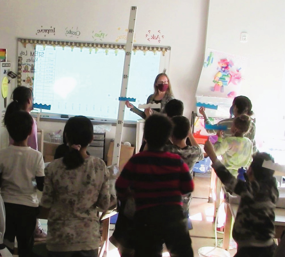
The class models a river.
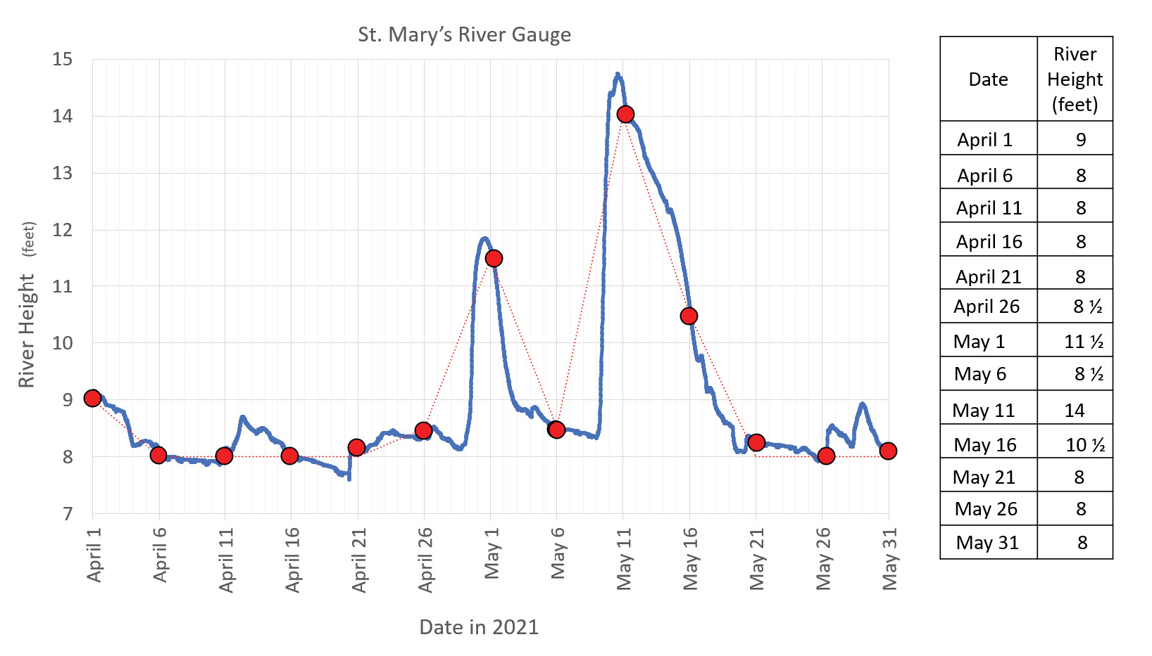
Graph of river height.
- “We wouldn’t have noticed that [the river height] is actually not just 14 feet. It’s about 14 and three quarters.”
- “The blue line has little spikes and dips between the points ... it tells how much the river went up and down between the red points.”
Working with the classmate next to them, students were given four photos of a river taken by a webcam at the site of a river gauge. The photos were identified by a shape so students could easily refer to them (triangle, square, diamond, star). The students observed the photos and readily recognized the images were of the same scene, and that both short-term changes (e.g., sunlight, turbidity) and long-term changes (e.g., amount of foliage) could be identified. Importantly, among these observations were those indicating differences in river height, such as changes along the riverbanks and water level on exposed parts of plants.
The student pairs were then given a hydrograph with four data points marked and were asked to infer which photo matched each data point based on their observations. As students shared their ideas, they were encouraged to support their claims about the matches using evidence. For each data point, a student volunteer shared which they thought was the associated image, giving their evidence and reasoning. Other students responded, first with agree/disagree hand signs to increase involvement, and then by providing their own explanations, sometimes offering different rationales for the same conclusion, and sometimes giving different inferences and their evidence for those:
- “I think the diamond should be 3 because it’s just a little higher than number one and if you look at the hydrograph, it calms back down and it comes back, but it doesn’t calm down fully.”
- “I think it is the diamond…because if you look at the diamond, you can see it’s lower…than the other two and higher than one. And so then you can see most of the tree in there.”
- “I think its… the diamond… you can see the ground, but on the star you just see it eroding away, it turning into …whatever, dirt.”
Days 2–4: How Water Moves
To understand the Ellicott City flood, it is critical for students to know about how water moves through urbanized areas. Therefore, we focused lessons on days 2–4 considering the question, “How does water move in natural and urban environments?” Students used models to investigate how water moves to a river, the relationships between rain events and river height changes, and factors that affect water movements. This includes the effect of land cover that allows water to infiltrate (pervious surface) or not (impervious surface). To support understanding of new terms, especially given the high English-language learner population in some classes, terms such as pervious and impervious were introduced using a “total physical response” method, which relies on hand gestures to reinforce the meaning of the terms (Inciman Celik, Cay, and Kanadli 2021).
On day 2, students worked in table groups to create a riverbank model using parts of an Awesome Aquifer Kit (see Online Resources). Pushing the gravel to one side, they simulated a riverbank and riverbed. Students then poured colored water onto the riverbank and observed the path it took to get to the riverbed, which allowed the introduction of the concepts of groundwater flow and surface water flow. A whole-class discussion was facilitated using open-ended prompts (e.g., “Share what you observed.” “What did you notice?”) and encouraging students to clarify their thinking by providing evidence for their statements about how the water moved.
Instructor: Who can tell me how the water got from the riverbank to the riverbed?
Student 1: The water goes through the rocks and then goes down.
Instructor: Is that what you expected? [Many students respond “yes.”] Who can tell me more about that?
Student 2: The water went through the cracks of the rocks and slowly went to the riverbed.
To allow students to investigate how surfaces impact the method and timing of water travel to a riverbed, we developed an innovative use of stream tables (Figure 3). Student groups simulated rain falling by pouring water from a 2L bottle with holes drilled near the top. Using this “rain bottle,” each group simulated rain falling uphill from the riverbed, timed how long it took for the river to begin flowing, and observed how the water moved into the riverbed (i.e., as surface water flow or groundwater flow). The model landscape was made of sand with the top third covered with either pervious (green cloth) or impervious (gray vinyl) surface. Using the models, students observed that water moves primarily as groundwater through pervious material and as surface water flow over impervious material. Their understanding was further evidenced by their depictions on diagrams and within class discussions. For example, one student stated, “At first, it felt like it wasn’t working because the water kept going into the ground and we couldn’t see it, and then it started like, coming out into the riverbed, then like, we could see it.”
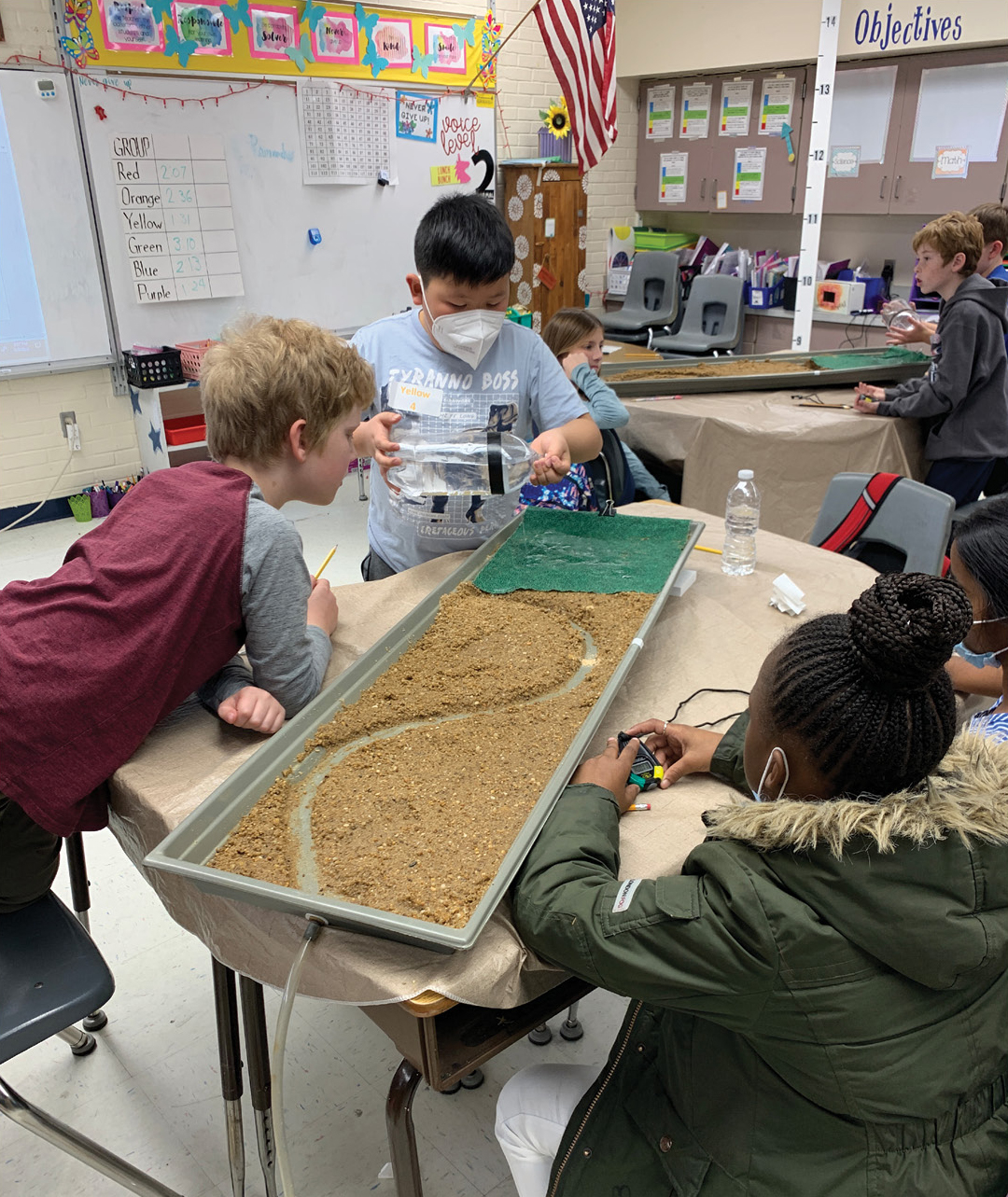
Using the stream table.
The water travel times students measured varied from 2 to 10 minutes for the pervious surface and less than 2 minutes for the impervious surface. The differences between water travel times led the students to fruitful discussions about effects of conditions such as land cover, prior rainfall, and terrain—each of which is connected to characteristics of flash floods.
Interspersed throughout work with the models, students explored data that contextualized the concepts in relation to locations on two rivers. We segmented the lessons so students developed familiarity with one river location, a forested and agricultural area around the Pocomoke River (day 2), and then added comparisons to a location on the second river, a section of the Patapsco River that is downstream from Ellicott City, which is an urban area (day 4). Each river was introduced with a flyover video made using Google Earth, which travelled from the students’ school to the river gauge location. Students were enthusiastic about seeing their school in the flyover, and this approach supported students’ qualitative interpretation of data in aerial images. Students’ understanding of the real-world contexts was further supported using data shown in circle graphs of pervious and impervious surface amounts around the rivers, which were created using ArcGIS land cover data. These applications of modeling helped students develop their understanding of the value of the developing and using models.
Once the foundational idea that river height can change was established, students were asked to annotate an 11-day hydrograph, noting anything that drew their attention. This allowed the instructor to assess ideas that students found interesting and/or what they had questions about. Many of the students marked the high points on the hydrograph as catching their attention, and many also noted that some graphs sloped gradually while others had abrupt changes (Figure 4). Students also used the annotated hydrograph to make inferences about when it had rained. Students generally inferred that rainfall occurred in connection with a rise in river height, though the timing of those events was in many cases unclear to them prior to working with the stream table.
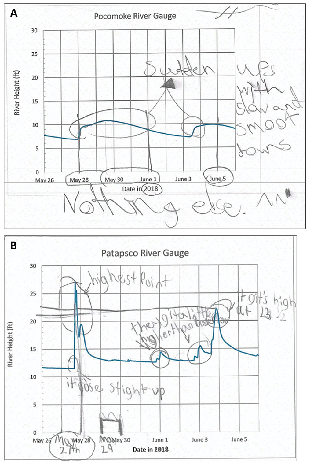
Student analysis of hydrographs.
There were several aspects of these lessons that called on students to recognize relationships between variables. For example, students were provided graphs that showed one variable at a time (i.e., precipitation, river height) and then in combination with each other as a dual plot (Figure 5). To support learners of different ability levels with these higher order interpretations, we developed strategies that used physical and auditory elements to help interpret the data. For example, to aid students’ understanding of the relationship between river height and precipitation, we created an animation of a horizontal indicator moving slowly across a dual plot of rainfall and river height. Students were asked to say “rain” and clap when the graph showed the rain starting, and then pat their legs and say “river” when the graph showed the river starting to rise. The difference in the motions and sounds helped them identify the delayed effect of the rain on the river, and to consider the amount of the time that passed between the start of the events.
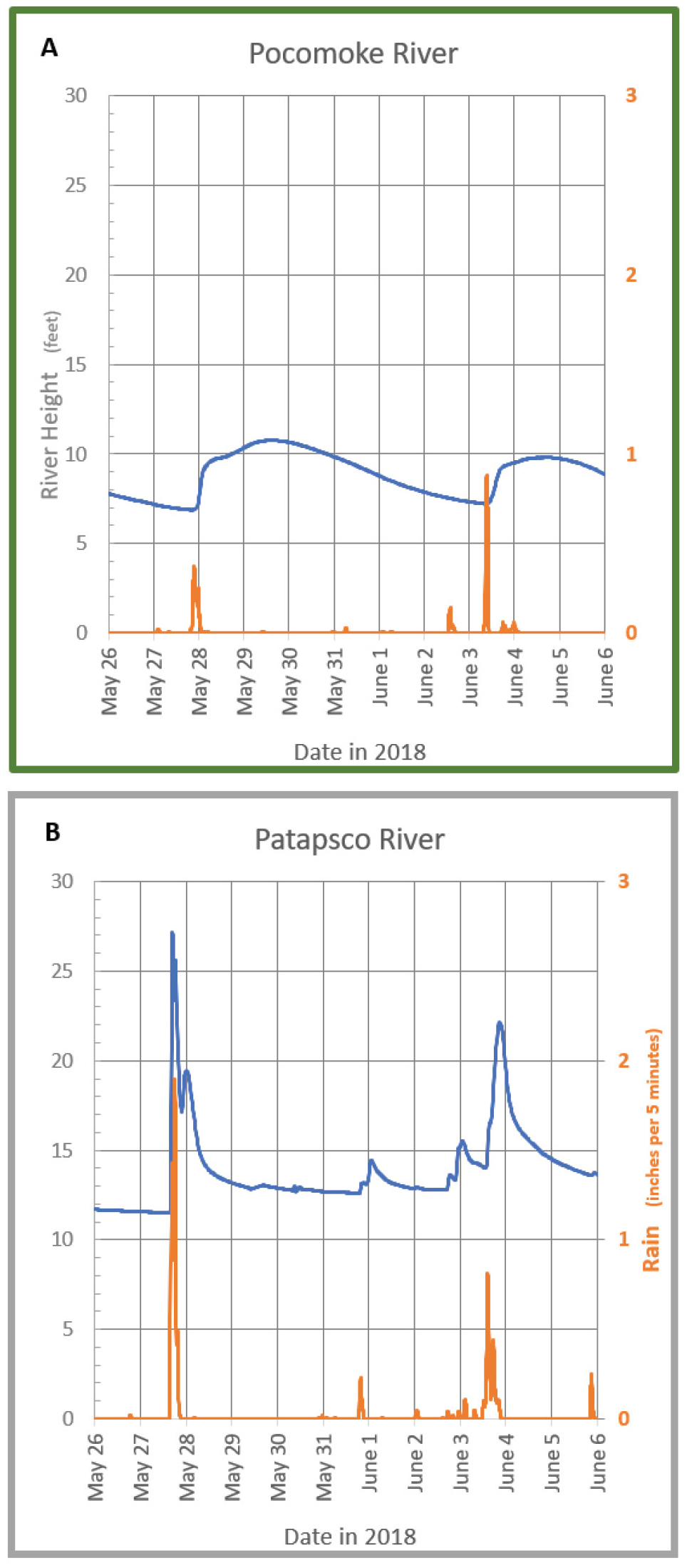
Dual plot graph.
By the end of day 4, through data-related support and the stream table experiences, students readily recognized several concepts necessary to understand flash flooding, such as that rivers near pervious surfaces have a longer time between rainfall and change in river height than rivers near impervious surfaces:
Instructor: “Our stream tables were set up so we had one with all pervious surface, and one with all impervious surface. What did you notice about what happened with the different surfaces?”
Student 3: “It was different because with the other one, it went down and came out like through the sand, but on this other one, it came out from the top.”
Instructor: “Can anyone use words we learned today to describe what she was talking about?”
Student 4: “So, when we didn’t use the thing to cover up the pervious part, um when we poured on the water, it would be pervious because the water was going through the sand to make the river.”
Instructor: [To Student 5] “What were you going to add?”
Student 5: “I noticed that when we had the non-pervious, or impervious surface, it went way faster. My prediction was that because the soil was covered and water moved from the place where it was like surface water ... that’s why I think the groundwater was lower and the surface water was more.”
After exploring how water moves in natural and urban areas, students were primed to make connections between human activities and the incidence of flooding. We introduced surface water flow mitigation strategies such as infiltration basins, porous pavement, and rain gardens that can be installed in areas with high levels of impervious surface. Students watched another video of the Ellicott City Flood to identify the prevalence of impervious surfaces, and we discussed the importance of mitigation strategies and how they might help.
Students ended the lesson sequence analyzing aerial images and pie charts of pervious and impervious land cover of their community, which they used to consider if and where mitigation strategies might be useful. By making connections to the students’ community, the content was more relevant and reinforced the understanding that flooding can happen regardless of a river being nearby, as well as that communities can act to reduce risks from flash floods.
Conclusions
The inclusion of a specific natural disaster, hands-on models, and other multimedia experiences engaged students to learn about rivers and flooding. It was clear through verbal and written comments that students understood concepts related to flooding (water movement, land cover, etc.) and were able to reason with data—both their data from the stream tables and professionally collected data about river height and rainfall. These lessons provide many possibilities focused on community-relevant anchoring phenomena related to natural hazards, how human activity affects the incidence of these hazards, and how people can work toward reducing the occurrence, severity, and impact of natural hazards.
Acknowledgments
This material is based upon work supported by the National Science Foundation under grant numbers 1906264, 1906286. Any opinions, findings, and conclusions or recommendations expressed in this material are those of the author(s) and do not necessarily reflect the views of the National Science Foundation. The work was undertaken by the American Geosciences Institute and the Education Development Center’s Oceans of Data Institute.
We would like to thank the education and science professionals who provided input into this work. Several teachers in three school systems contributed a great deal to this work, but unfortunately cannot be named here for reasons of confidentiality in research. Thanks, too, to Dr. Jonathan J. A. Dillow, Hydrologist at the USGS MD-DE-DC Water Science Center who generously reviewed the lessons from a scientific perspective, and Dr. Claudia Burgess for her reviews and advice related to mathematics instruction. Our advisory panel members also graciously offered insights and guidance that improved many aspects of the project, including the instructional design and delivery.
Online Resources
Groundwater Foundation: Awesome Aquifer https://awesomeaquifer.com
Lesson plan, slides, model setup, and handouts www.americangeosciences.org/streams-of-data
Lauren E. Brase (LBrase@americangeosciences.org) and Lindsay C. Mossa are education specialists, and Edward C. Robeck is director of education and outreach, all at the American Geosciences Institute in Alexandria, VA.
Climate Change Climate Science Earth & Space Science Phenomena Elementary