
feature
Modeling the Melting of Permafrost
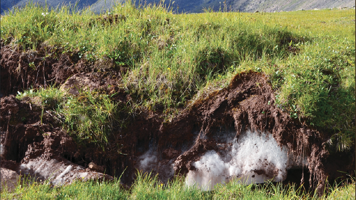
Permafrost is any soil or surface deposit in an Arctic or alpine region at some depth below the surface at which the temperature has remained below zero degrees Celsius (32 degrees Fahrenheit) continuously for a long period of time. Although most of us will never see permafrost, it is relevant to our lives in many ways. The amount of carbon dioxide and methane stored in permafrost is nearly twice the amount in the atmosphere and, as the ice melts, these greenhouse gases escape, warming our planet (Markon, Trainor, and Chapin 2012). Locally, the land surface is disturbed, the water cycle changes, and ecosystems are disrupted (National Research Council 2014; Cho 2018). Changes to the atmosphere are invisible and permafrost formed in distant polar regions, so it is difficult for people to see changes that result from melting permafrost. Building a model in the classroom connects students with a visual representation of permafrost and provides observations of physical and thermal changes.
Students begin the lesson by examining why the melting of permafrost matters. Next, they construct a physical model of permafrost in the classroom that provides insights through observation, data collection, and comparison to authentic permafrost data. In addition to constructing a realistic physical model, students use technology to measure temperature. The lesson concludes with students interpreting data from Alaska to identify patterns and estimate the rate of change.
Thermochron iButtons—small, round (1.5 cm), thin (0.4 cm) data loggers that contain a battery—are central to our model. Thermochrons record temperatures at regular intervals over days or weeks. They are excellent for science investigations. Huff and Lange (2010) used thermochrons in snow pits to investigate how temperature and snow density varied over time with their students. Huff and Lange noted the excellent opportunity for students “to use data as evidence to construct their explanations” and to “synthesize their understanding as students participated in discussions about their data and used this information to develop and refine their emerging theories about snow.” (2010, p. 41)
Getting Started
We used photos as prompts to reveal prior knowledge and misconceptions (see Useful Photos for Permafrost in Online Connections). Figure 1 (see Online Connections) provides useful questions and the responses below reflect the most common answers from students. Permafrost is an excellent example of Earth systems, connecting soil (geosphere), ice (hydrosphere/cryosphere), plants (biosphere), and air (atmosphere). Unfortunately, in many regions, permafrost is unstable and starting to melt. In most U.S. locations, students don’t have ice in their soil; only students in Alaska have permafrost. Potential problems caused by melting include flooding and uneven ground. Although students in Alaska might be directly affected by melting permafrost, coastal communities will be influenced by rising sea level, and all students are impacted by a warming atmosphere accelerated by the release of greenhouse gases once trapped in the ice.
Why Permafrost Matters
Melting permafrost affects people, wildlife, the land surface, and the atmosphere (Welch 2019). We introduced our students to the importance of permafrost using the lesson of Holzer (2011). Students began by visiting the National Snow and Ice Data Center (NSIDC) website to construct a definition of permafrost and read oral history accounts from Indigenous people. For example, the Chukchi communities in Siberia live in one of the coldest inhabited places on Earth. In this area, the melting of permafrost has disrupted the courses of rivers and caused lakes to disappear. In response these people moved homes away from eroding river banks, found new sustainable fishing lakes, and relocated their reindeer herds.
Next, students used Google Earth and the NSIDC file on permafrost to explore the types of permafrost and their distribution. Last, using the Data Visualization tool from the NOAA Earth System Research Laboratory, the students interpreted a time series of methane concentration from Barrow, Alaska. Methane has a global warming potential 28 times greater that carbon dioxide (U.S. EPA). As students progressed through the lesson, they observed that a warming atmosphere leads to melting ice, land subsidence, rising methane levels, and dramatic changes within a century.
Building the Model
Building the model is easy and fun. We guided our students and let them do the work. Alternatively, when pressed for time, we assembled the model prior to class.
Teacher Preparation: Be sure to activate the thermochrons and set them to measure every 10 minutes. With all the materials ready to use (see Materials List), construction takes about 20 minutes. We labeled our thermochrons (1–10) with a permanent marker to avoid confusion. We used scoria, garden soil from the landscape store, and crushed ice from the cafeteria.
Student construction of the model: Start by adding a 3 cm thick layer of scoria uniformly across the bottom of the aquarium. Place thermochrons 1 and 6, one quarter and three quarters along the length of the aquarium (see Figure 2), near the center. Add another 3 cm of scoria to bury the thermochrons. Place thermochron 2 above number 1 and thermochron 7 above number 6. Add another thin layer of scoria, just enough to bury the thermochrons. Add a 1–2 cm layer of crushed ice. Smooth the ice to a uniformly flat surface. Place thermochron 3 above 2 and 8 above 7. Add another 2–3 cm of ice. Place thermochrons 4 and 9. Cover with a 1–2 cm layer of ice and smooth. Cover the ice with a 1–2 cm layer of soil. Place thermochrons 5 and 10 in their positions. Bury with 2–3 cm of soil. Place the cardboard divider as a vertical barrier to the light across the middle of the aquarium. Place the lamp about 20 cm above the soil (a ring stand might help).
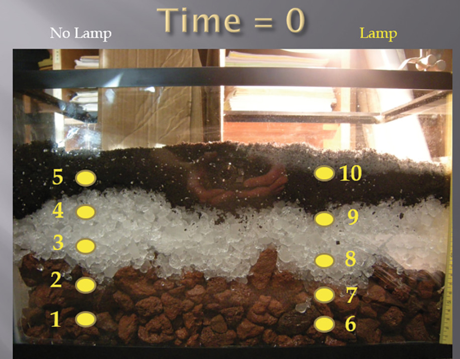
Model design and placement of thermochrons. Note the ruler along the right margin.
Running the Model
Students constructed their knowledge about permafrost by making observations, collecting data, interpreting patterns, and making predictions. We began the experiment at the start of the school day and let it run all day. We introduced later classes to the model setup. Each class took a photo of the model and noted the time. After 8 or 9 hours the model changed considerably (Figure 3a and b) and nearly all the ice melted on the heated side.
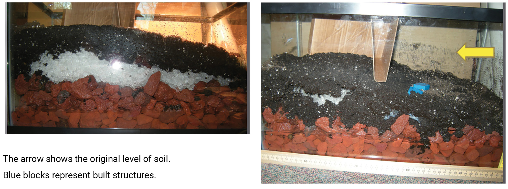
(a) Photo of the assembled model after five hours (b) photo of the assembled model after eight hours.
After the experiment was completed, students retrieved the thermochrons and cleaned up the model. To reuse the soil, place it on a tray to dry; alternatively, place it in an appropriate place outside. We rinsed the soil off the scoria, allowed it to dry, and saved it for the next time. The aquarium was rinsed, dried, and stored.
Next, students reduced the data. They rinsed and dried the thermochrons. Each thermochron was placed in a reader and the accompanying software pulled off the data (Figure 4). We pasted the data into a spreadsheet, separated by each hour, which provided 6 to 9 data sets. Small groups of three or four students reduced the measurements made every 10 minutes to define an average for each hour (1 to 9) or group to hour 1, hours 2 and 3, 4 and 5, 6 and 7, hour 8, and hour 9. The students then combined their data to define a complete picture of the temporal changes in temperature on both sides of the model for each thermochron (Figure 5). Next, each student plotted the class data to make the patterns visible (Figure 6; also see link to Blank Graph in Online Connections). Depending on your students’ skills, data reduction can take up to one hour; plotting and interpretation takes about one hour.
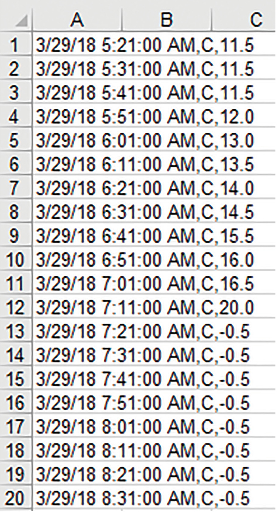
Sample of raw data from a thermochron.
Temperature in °C and measurements taken every 10 minutes. The thermochron was buried in ice just after 7:11 a.m.
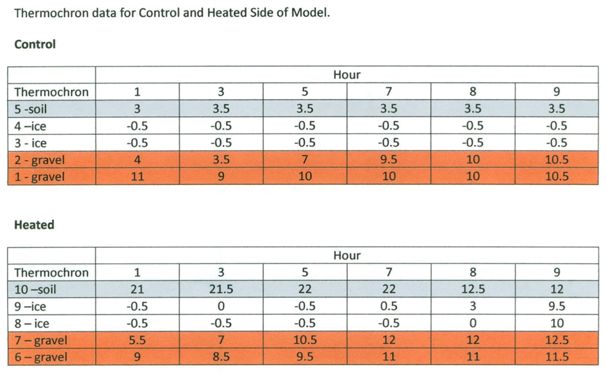
Sample of reduced thermochron data for students to plot.
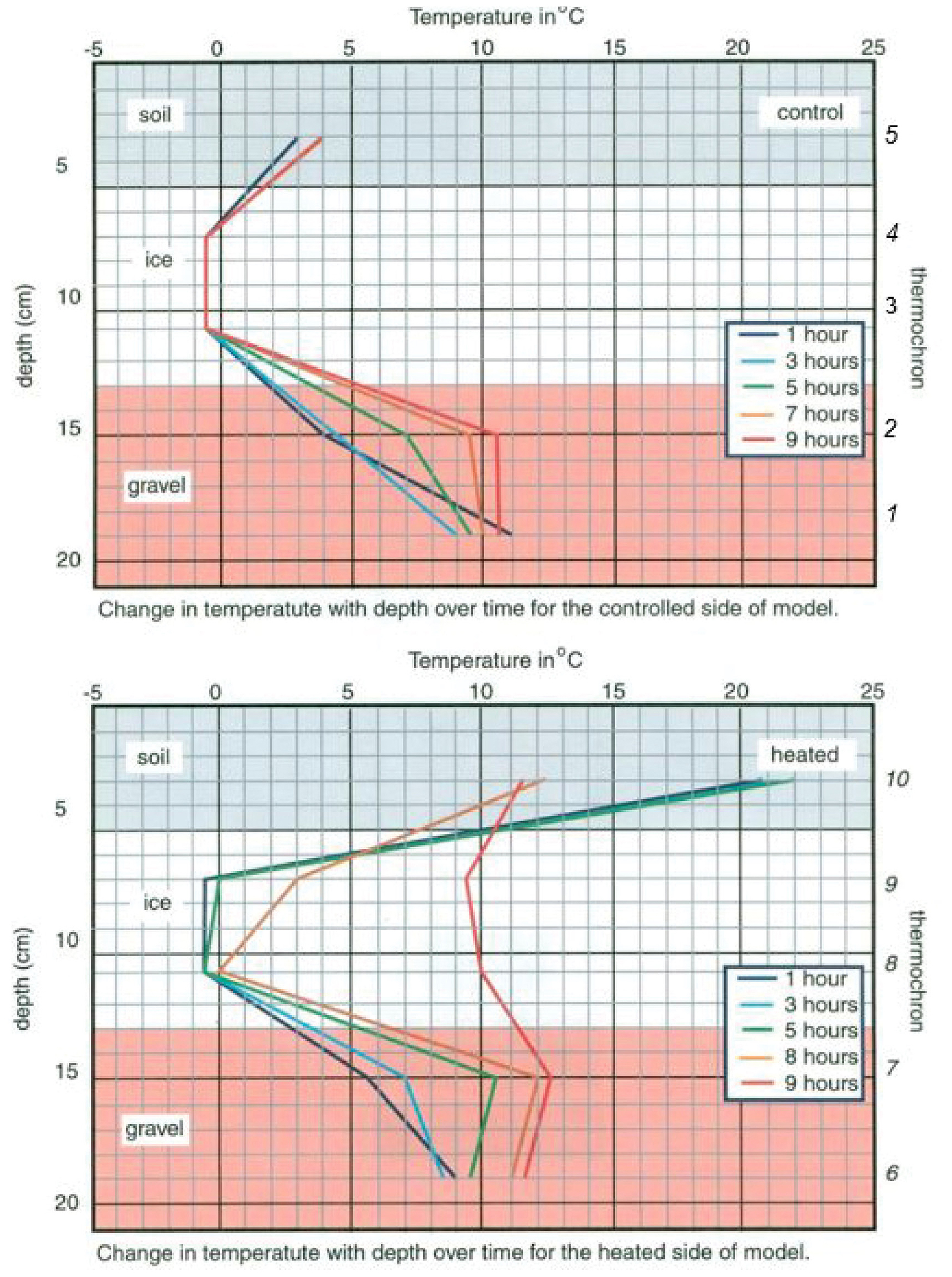
Graphs of student data.
Top: Ice remains stable and soil and scoria show a slight temperature increase. Bottom: Ice remains stable for about five hours then melts. Soil temperatures started high and then decreased as soil settled lower. Scoria layer became progressively warmer.
Interpreting the Results of the Model
Next, students interpreted the patterns that emerged from the data. We provided a set of questions to guide the students and lead class discussion (Figure 1). A glance at the model at the end of the experiment (Figure 3b) showed significant differences. Students coupled their visual observations with the reduced data to describe changes over time. We offer a sample set of observations based on data we commonly collected; your data set will be slightly different but the same patterns should emerge. The abilities of students to answer these questions varied. For example, some students missed subtle visual clues of the heated-side of the model sinking away from the lamp. Other students had difficulty in calculating rates of change. It helped to have students work in pairs or groups of four to answer the questions. As needed we guided students in setting up some calculations. We used the students’ responses to the questions about the model as a summative assessment.
For the control (no added heat) side of the model, the soil heated up only 1°C in nine hours. The ice remained stable, below freezing. The scoria layer became progressively warmer from 3°C up to 11.5°C, indicating heat was also absorbed from the base. In contrast, for the heated side of the model, the soil started out much hotter, about 21 or 22°C. After nine hours it cooled to about 12°C. The ice remained stable for about five hours but then the layer started to warm progressively, from 3°C to about 10°C. The upper part of the scoria layer showed a progressive increase in temperature, up to 12.5°C. Most of the change was in the last three hours.
What did the model predict about permafrost areas as the surface warmed? The two temperature profiles are different. The control showed no change in ice and suggested stability. The heated side showed change, especially warming, and, over time, loss of ice and uneven settling of the land surface as the ground sank. On the control side, the land settled very little. On the heated side, the land surface lowered significantly as the ice melted below the soil. There were cracks in the surface.
What’s happening in the Arctic?
To elaborate on changes to permafrost, we placed our students in a real-world scenario. The model revealed the influence of warmer surface temperatures on ice at depth, but is it realistic? Temperature loggers were deployed in northern Alaska to depths of 60 m at 16 locations along a north-south transect (Osterkamp 2005). A set of data is presented in Figure 7. Depending on your students’ skills and the time available, you can have students plot the data or project the graph for discussion. Questions to guide the students are provided in Figure 1 (p. 31).
All students recognized that the temperature data defined a general pattern of the permafrost getting warmer every year. The rate of warming was faster at shallow depths, about 3°C over 18 years, versus a 0.5°C increase near the bottom. Some students stopped after determining the change in temperature and had be reminded to calculate a rate of change. The pattern suggested heat was being added from the top and penetrating to the base of the permafrost. From 1985 to 2003, the permafrost was not melting because all the permafrost was below 0°C and it remained solid. A few students needed to be reminded that ice melts above 0°C.The base of the permafrost would begin to melt in a few decades. At a rate of about 3°C per 18 years (~1°C every 6 years) permafrost at 10 m depth would begin melting in about 36 years, about the year 2056 (roughly when current high school students are as old as their parents!). At 50 m depth the ice warmed from -8.2 to -7.7°C over 18 years, a rate of about +0.027°C per year. At that rate, it would take about 285 years to melt to the base of the permafrost (7.7°C × 1yr/0.027°C). Once the students had the correct rate of melting, they quickly calculated when deeper layers would melt. We assumed the same conditions as 1985 to 2003, which seems overly simplified. So, the 285 years would be a maximum; the changes will probably happen sooner. As the overlying, shallow layers melt, the rate of melting at depth would increase and migrate to deeper levels. Note: about 285 years ago U.S. historical figures Paul Revere and John Adams were born. If we used the average rate for all the layers, it would take about 92 years to melt the permafrost currently at the base (7.7°C × 1yr/0.083°C). In about 92 years the great grandchildren of the current high school students will be in high school. Based on these simple calculations the students realized that much of the carbon stored in the Arctic will be released to the atmosphere in their lifetime. Considering that the students practiced analyzing data of melting permafrost from the model, their interpretations and calculations from the Arctic data can serve as a formative assessment.
Was this a good model?
At the end of the lesson, we ask students to connect back to the physical model and compare their data with the patterns in the Alaska data (see questions in Figure 1). In some ways the model did not match the real world. For example, cooling was caused by the soil/land surface being lowered away from the lamp, so the temperature decreased. In a real system, the land surface would not move away from the atmosphere.
The model was good in that it mimicked the observed temperature patterns of the real world: additional heat caused the permafrost to melt, temperature change mimicked real-world data, rates of change can be calculated, the land surface was disrupted, and the water cycle was altered.
However, the model is limited in some ways: size and scale (limited in lateral continuity, thickness/depth), designed (not a natural system), heat source (lamp, not the atmosphere), temperatures (actual temperatures in Alaska were much colder), time (ice melted in hours, not over decades), and it was a closed system (the water is trapped in the model).
Extension
Our model assumed the atmosphere in the Arctic is warming. PBS LearningMedia provided data-rich activities and videos as part of their “Alaska Native Perspectives on Earth and Climate” collection that includes interpretation of air temperature (see https://www.pbslearningmedia.org/collection/ean/). The Third National Climate Assessment offers resources on a variety of impacts including the impact on native communities (see https://www.climate.gov/teaching/national-climate-assessment-resources-educators/alaska-region).
Permafrost is already melting in some places. Reading news stories provides a literacy connection with the science lesson and demonstrates local impacts such as “Canada’s Permafrost Is Thawing 70 Years Earlier Than Expected” (Suleman 2019), “Arctic Circle sees ‘highest-ever’ recorded temperatures” (BBC 2020), and “Russia declares state of emergency over Arctic Circle oil spill caused by melting permafrost” (Weise, Zaiets, and Gelles 2020).
Conclusion
Experiments connect our classrooms to the real world. Developing a sense of the unseen, either methane in the atmosphere or ice in soil, is central to science and critical to acting on climate change. In this lesson, students gained skills and confidence by generating and interpreting their own data. Faced with similar real-world data students recognized patterns and predicted significant changes in Earth systems in their lifetime.
Online Connections
Figure 1. Questions to guide students’ thinking: https://bit.ly/3ojHkgH
Blank graph: https://bit.ly/3oiT4jk
Activities and time needed: https://bit.ly/34uO3Nz
Materials list: https://bit.ly/3h6sari
Why thawing permafrost matters: https://blogs.ei.columbia.edu/2018/01/11/thawing-permafrost-matters/
NASA Climate Kids at https://climatekids.nasa.gov/permafrost/
NRDC Permafrost: Everything You Need to Know: https://www.nrdc.org/stories/permafrost-everything-you-need-know
Interagency Arctic Research Policy Committee: https://www.iarpccollaborations.org/teams/Permafrost
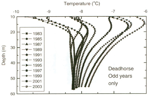
Observed changes in permafrost temperatures in Alaska from 1983 to 2003 in northern, Alaska.
Note: Ice remained stable over this time period but temperature increased at all depths but faster near the surface. From Osterkamp, 2005. Reprinted from Global and Planetary Change, v. 49, issues 3-4, Osterkamp, T.E., The recent warming of permafrost in Alaska, P. 187-202, 2005, with permission from Elsevier.
Stephen R. Mattox (mattoxs@gvsu.edu) is Professor of Geology at Grand Valley State University in Allendale, MI; Stephanie Duda is an elementary teacher and high school procto in Franklin, TN.
Earth & Space Science Phenomena Physical Science Science and Engineering Practices Technology High School