
feature
Using Climate Models to Learn About Global Climate Change
Investigating the Phenomenon of Increasing Surface Air Temperatures Using a Global Climate Modeling Approach
The Science Teacher—September/October 2020 (Volume 88, Issue 1)
By Devarati Bhattacharya, Kimberly Carroll Steward, Mark Chandler, and Cory Forbes

Since 1880, Earth’s average global temperature has increased by approximately 1.4 °F (0.8 °C). Approximately two-thirds of the warming has occurred since 1975 (Wuebbles, Easterling, Hayhoe, et al. 2017). Despite consensus about global climate change (GCC) within the scientific community, students struggle to comprehend
- why temperatures are increasing globally
- at what rate this change is occurring, and
- how climate scientists predict Earth’s future climate.
These challenges are due, in part, to the abstraction inherent to understanding GCC, a phenomenon that occurs over long periods of time (past and future), and over large regions (regional and global). With the adoption of the Next Generation Science Standards (NGSS Lead States 2013), GCC is emphasized at the secondary school level, with a focus on analyzing and understanding the evidence for GCC (HS-ESS3-1), climate modeling (HS-ESS2-6, HS-ESS3-5), and the impact of humans on the environment (HS-LS2-7, HS-ESS3-6).
However, learning opportunities that emphasize developing students’ understanding of the basic science underlying GCC, such as the greenhouse effect and the carbon cycle (Zangori, Peel, Kinslow, Friedrichsen, and Sadler 2017), may not fully address the temporal and spatial aspects inherent to this phenomenon (National Research Council [NRC] 2010) and teachers may not have access to high-quality curriculum materials that could help in addressing these challenges (Colston and Ivey 2015; Herman et al. 2017; Plutzer et al. 2016).
To enhance teaching and learning about Earth’s climate and GCC in secondary science classrooms, we are engaged in a four-year, NSF-funded project to develop, implement, and evaluate a new four-week curriculum module grounded in the use of a data-driven, computer-based climate modeling toolkit—EzGCM (see Forbes et al. 2020).
Instructional approaches focused on investigations grounded in climate data have been successful in improving students’ understanding of the global warming phenomenon, as well as the methods scientists use to develop the evidence (e.g., Holthius, Lotan, Saltzman, Mastrandrea, and Wild 2014). However, it is challenging to obtain, analyze, understand, and present large scientific data sets and complex computer models in the classroom. Tools such as EzGCM make modeling and big data more accessible to students and more appropriate for classroom teaching and learning. However, if not integrated meaningfully, students’ interactions with these data and models remains superficial (Bowen and Rodger 2008). In this article, we describe our approach to using models to support students’ reasoning about Earth’s climate and GCC through the use of EzGCM.
The EzGCM Climate Modeling Toolkit
Global Climate Models (GCM) are one of the primary tools that scientists use to study GCC by simulating both historical and future climate change. Representing Earth’s atmosphere, oceans, and land, GCMs attempt to account for a vast array of Earth system processes using fundamental physics (conservation laws and state equations) combined with parameterizations, which describe physical phenomena empirically (equations based on observations). Over the past two decades, researchers at Columbia University and NASA have created user-friendly software tools rooted in authentic NASA climate research, making the science of climate modeling more accessible to students and teachers.
The most recent of these tools—EzGCM—brings climate modeling to secondary school settings using cloud-computing resources and web-based interfaces that run on Chromebook and tablet computers. Through EzGCM, students engage in authentic methods of research, including
- running simulations
- processing model output into meaningful scientific data sets
- creating useful scientific visualizations, and
- analyzing student-generated data to improve comprehension of key climate concepts.
Students can make robust data-driven and model-based predictions about future climate change and, combined with a better understanding of Earth’s climate system, come to their own conclusions about GCC based on results they themselves generate. EzGCM is a gateway toolkit that can help high school students better understand GCC and make sense of the major national and international climate assessments that inform and guide climate change policy.
Instructional plan
This 1-week investigation is part of a 4-week curriculum module (Table 1) comprised of ten lessons designed to foster students’ engagement in scientific modeling using EzGCM to develop understanding of core climate-related concepts (DCI) as prescribed in HS-ESS2-2 and HS-ESS3-5. The investigation requires the following materials:
- Laptops or Chromebook or computer stations checked out in advance. Students can work in groups of 2-3 to accommodate a 1:3 computer ratio.
- Internet Availability and access to the EzGCM toolkit.
| Table 1. Unit calendar. | |||||||||||||||||||||||||||
|---|---|---|---|---|---|---|---|---|---|---|---|---|---|---|---|---|---|---|---|---|---|---|---|---|---|---|---|
|
To make this content accessible to English Language Learners (ELLs) and students with Individualized Education Programs (IEPs), we integrated the following practices into the curriculum and instruction
- Providing vocabulary lists, dynamic visuals, and graphic organizers with every lesson.
- Providing rubrics, correct answers and sentence frames such as “What I saw was____” and “this evidence comes from (graph) and the (reading)__” to help students in sensemaking.
- Leveraging opportunities to run and practice the climate model in multiple lessons, often for increasing efficiency of the process of extracting relevant data.
- Using formative assessments for evaluating both learning of science and language through developing of predictions and explanations.
- Using formative assessments to help teachers to identifying gaps between science and language understanding.
- Encouraging students to select geographical locations of their own choosing for investigations to capitalize on their prior knowledge about Earth’s climate.
This activity is designed for students to investigate the phenomenon of “increase in global average surface air temperatures” and its relationship to concentrations of atmospheric carbon dioxide, through the use of a global climate model (ESS2.D, ESS3.D). The model provides students access to big data and climate-based experiments to address the driving question, “Why does it feel like the weather is getting hotter each year?”. These data-based investigations afford students opportunities to use authentic modeling tools to make claims about climate-related concepts (DCIs) through the lens of multiple CCCs (Table 1)
The investigation begins with students divided into groups of 2-3 to make a claim about the relationship between atmospheric carbon dioxide and global average surface temperatures. For this purpose, the teacher encourages students to use their prior knowledge about the Earth’s climate and the phenomenon of GCC and provides a format for making claims such as, “Surface air temperatures increase as carbon dioxide increases in atmosphere.” Students also make a prediction about average surface temperature in year 2100. The teacher records students’ claims and collects students’ ideas about the relationship between observed atmospheric carbon dioxide concentrations and average surface temperatures in a graphic organizer.
As the investigation progresses, the EzGCM tool allows students to conduct multiple experiments (SEP-using models), where they collect and analyze evidence that one causes another. Students are also able to select parameters influencing Earth’s climate other than those described in this activity. This model-based analyses allows students to evaluate their initial claim and prediction (SEP-analyze and interpret data, use models) using data-based evidence. They are able to observe patterns (CCC-observing patterns) in the graphs and visualizations to establish relationships (CCC-stability and change) in the behavior of various parameters that impact Earth’s climate.
Here we emphasize one activity from the curriculum (Table 1). This particular investigation focuses on two parameters: surface air temperature and carbon dioxide concentrations. At the end of this investigation students are able to:
- Identify trends in visualization of surface temperature and atmospheric carbon dioxide generated using EzGCM (SEP analyze and interpret data).
- Establish the correlation between the concentrations of atmospheric carbon dioxide and the increase in global average surface temperatures (DCI-ESS2.D: Weather and climate; CCC Patterns).
- Posit evidence-based claims and predictions about rate of change in global average surface temperature and atmospheric carbon dioxide (DCI-ESS3.D: Global Climate Change; CCC Stability and Change).
- Recognize and describe how scientists model and predict current and future climate using global climate models (DCI-ESS3.D: Global Climate Change).
Part 1. Exploring Earth’s global average temperature increase using EzGCM
The purpose of this activity is to help students generate evidence for GCC by running two of the computer climate simulations provided in EzGCM and comprehend the phenomenon of increase in average surface temperatures (SEP-Analyze data using computational models, ESS3.D). Working in groups of 2-3, students brainstorm the responses to the question “How can we explain the phenomenon of global increase in average surface temperatures?” They record their responses in a graphic organizer. Students then access EzGCM model through a website (www.ezgcm.org) where they observe and learn about the features of the climate model. Teachers guide students in understanding the features of the model and compare the simulations or experiments provided by the model.
The simulation called Modern_PredictedSST is a climate model experiment that assumes atmospheric carbon dioxide remains constant at mid-20th century levels. This is called the Control Run, and it produces a stable climate against which other climate change simulations can be compared. The second simulation, called IPCC_A1FI_CO2, is a climate experiment based on a scenario in which atmospheric carbon dioxide gradually increases at a rate similar to the current rate of change.
Ask students to select Modern_PredictedSST and IPCC_A1FI_CO2 in the Simulations list (see Figure 1). Next ask them to, select Atmospheric Carbon dioxide and Surface Air Temperature from the Climate Variables list, followed by clicking on the Play button above the Simulations list. Both simulations are executed and data and plots showing changes in temperature and atmospheric carbon dioxide through time are generated. Teachers emphasize that humans are able to simulate climate data and predict future trends through the use of a climate model.
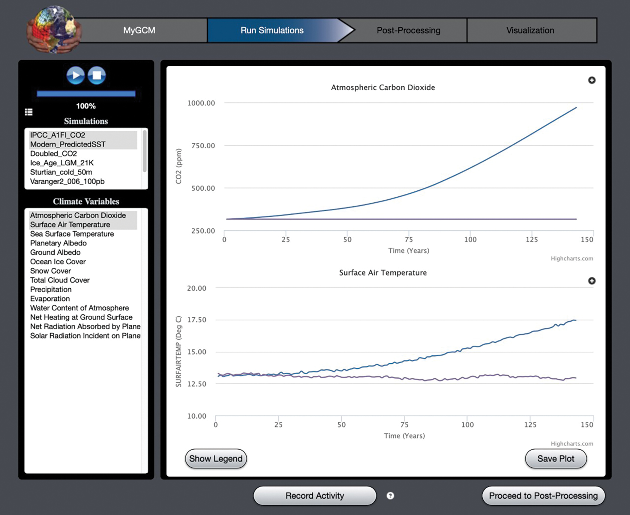
The Run Simulations component of the EzGCM toolkit.
Note: Pre-determine students’ working groups with criteria that allows for equal contribution. Help students as needed in accessing and navigating the EzGCM interface by asking leading questions, such as: “Were you able to access data and run the simulations?”
As students work in groups to explain trends and make predictions, the teacher supports students in developing their discourse as well as the science content.
Part 2. Investigating the correlation between average surface air temperature and carbon dioxide concentrations.
The purpose of this activity is to help students compare multiple types of data that are obtained from the EzGCM climate model. With teachers’ guidance, students explore time-series graphs obtained from the climate model in Part 1 (see again Figure 1) through small group and whole class discussion. The teacher asks students what they consider to be good evidence of relationships between variables? Students provide examples such as data from an experiment or data collected over a long period of time. Teachers can use the following questions to support students’ interpretation of the model-based data and sensemaking about DCIs and CCCs by examining time series graphs of two variables that change over time in the two different simulations:
- What information do these graphs provide? × and Y axes for both graphs and their respective units. Atmospheric carbon dioxide is measured in parts per million (ppm) and temperature is measured in Celsius. Time is measured in number of years from the beginning of the simulation. Both simulations run from January 1, 1958 to December 31, 2100, or 143 years. (SEP: analyzing and interpreting data)
- How does the rate of change in surface air temperature change through time in the two simulations? How does the rate of change in atmospheric carbon dioxide compare between the two simulations? Is the rate of change of these variables consistent from the beginning to the end of the simulations? Students should observe that there is much greater change occurring in both surface air temperature and atmospheric carbon dioxide in one of the simulations. The also should observe that in the simulation where carbon dioxide and temperature are changing the rate of change increases over time.
- How does the behavior of atmospheric carbon dioxide compare to that of surface air temperature in the control run (Modern_PredictedSST)? Similarly, how does surface air temperature change compared to atmospheric carbon dioxide in the climate change simulation (IPCC_A1FI_CO2)? Students should note if the variables change over time. Students observe and record that the trend lines for carbon dioxide follow the trends of surface air temperature in both runs, although the change is much greater in one of the two simulations.
Following this discussion, students revisit their graphic organizer and reevaluate their claims about the relationship between atmospheric carbon dioxide levels and surface air temperature.
Part 3. Preparing data for analysis by averaging and extracting simulated temperature output.
In this step, students perform mathematical functions on the data obtained from the model in order to extract optimal data to use as evidence to support their claims. Referring to Figure 2, ask students to select Modern_PredictedSST in the Simulations list, then select the range 2099–2100 in the Years list (or click on the Last 2 button). Next, click on the Average button below the list of years. A window opens showing a computer program is running on the cloud server. Within 30–60 seconds an average of all of the climate variables from the final two years of the simulation has been created and saved for analysis.
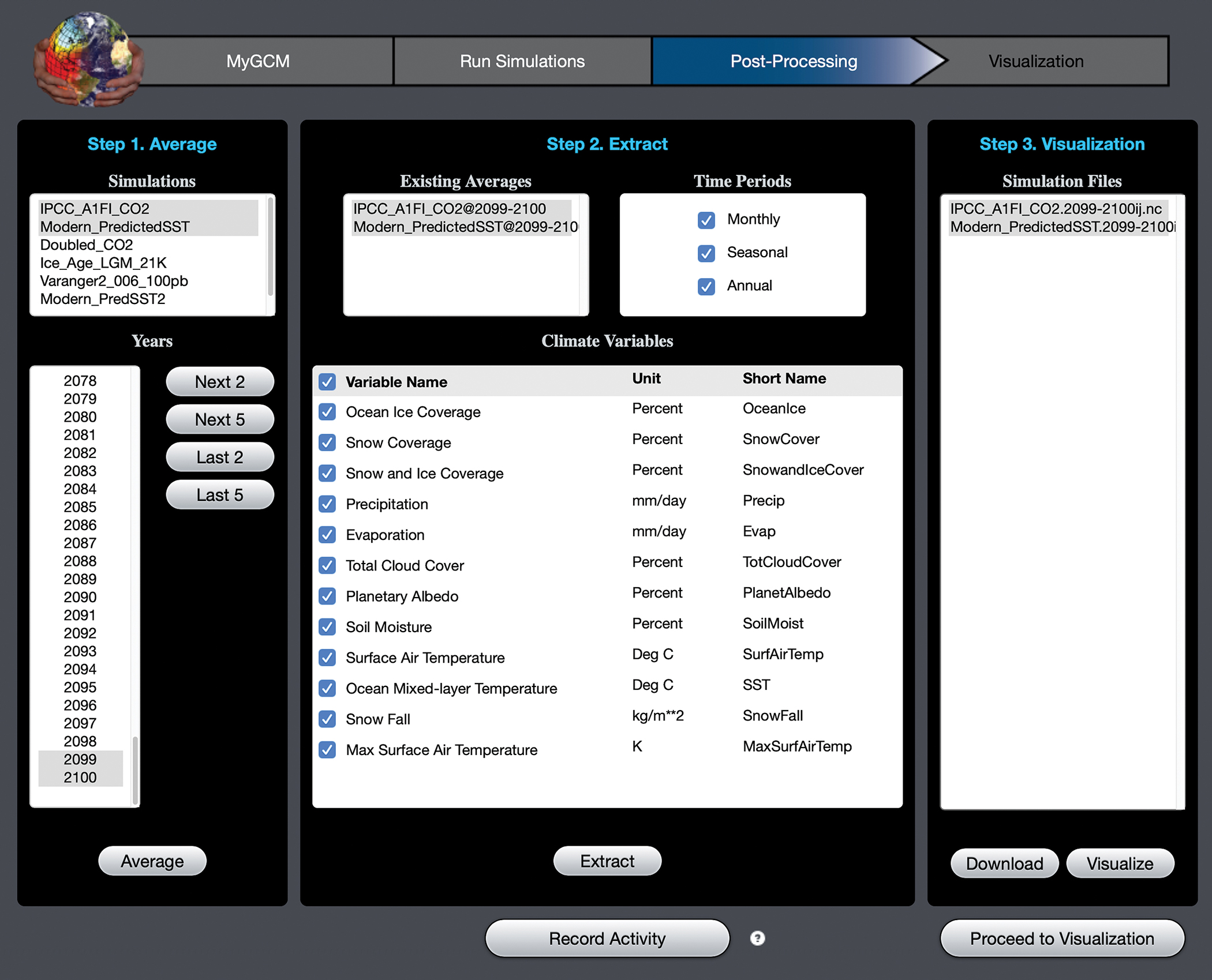
The EzGCM Post-Processing utilities.
Repeat these steps for the simulation IPCC_A1FI_CO2, then instruct students to turn their attention to the center Extract column. In the Existing Averages list, ask students to Select both Modern_PredictedSST@2099-2100 and IPCC_A1FI_CO2@2099-2100 and select Surface Air Temperature in the list of Climate Variables. Upon clicking the Extract button at the bottom of the column, another program runs and two items appear in the Visualization column on the right. Students select both of these Simulation Files and click on the Proceed to Visualization button at the bottom of the column.
At the end of this section, the teacher asks students “How do you know the data you extracted from the model is accurate?” Students revisit their claims and add information about the steps they engaged in to obtain their data-based evidence.
Part 4. Creating a scientific visualization of the simulated surface air temperature increase.
Students next use the EzGCM tool (Figure 3) to show processed data in the form of a visual temperature map. Ask students to look at the left column and select IPCC_A1FI_CO2 and Modern_PredictedSST in the Simulations list, SurfAirTemp in the Climate Variables list, and Annual in the Time Periods list.
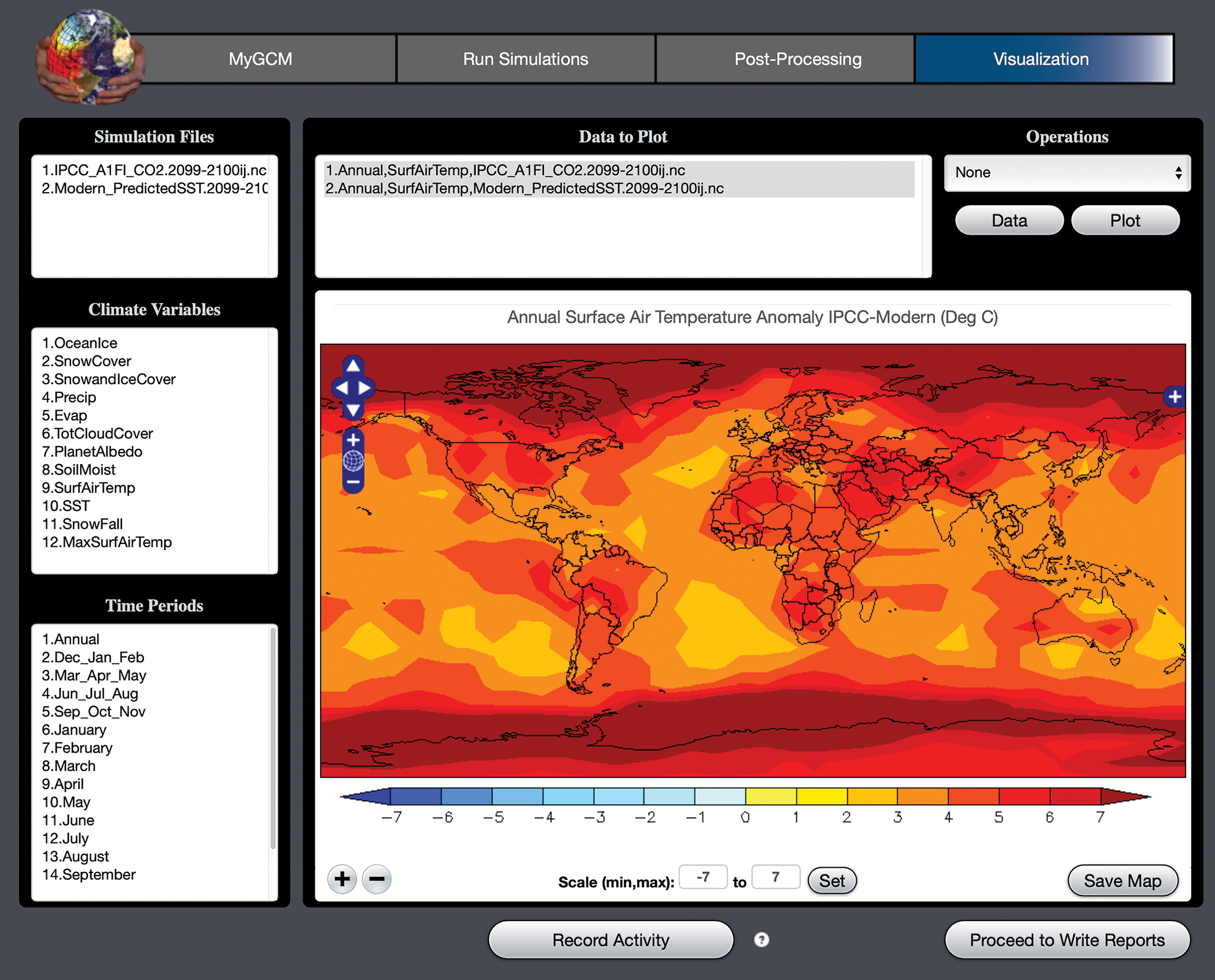
EzGCM scientific visualization tools.
Next, under Data to Plot (top center), select both data sets 1 and 2 and then find the difference between the two data sets using the Operations menu to choose Top— Bottom and click on the Plot button. Differencing the data sets creates an anomaly map, which is how scientists visualize the amount of global warming predicted to occur by the year 2100 compared to a hypothetical future where there were no increases in carbon dioxide.
To better understand this map, ask students to set the Min and Max fields (below the colorbar) to—7 and 7 (units are °C). This has the effect of adjusting the center point of the colorbar scale to 0 °C. Now colors greater than 0 °C (right side of the colorbar) represent regions where temperatures have increased, while colors less than 0 °C are regions of cooling. Students then examine the temperature anomaly maps with varying levels of guidance as determined by the teacher. Teachers can support students’ sensemaking about DCIs and CCCs by asking them questions similar to those in Part 2:
- What information do these maps provide? Emphasize that this map is not just an image like an artist would create, but a scientific representation to visually express data and evidence. This visualization demonstrates that there is an overall increase in average surface temperature and that the amount of increase varies geographically. In addition, adjusting the scale on the colorbar changes the visualization, but does not change the underlying data. (SEP: analyzing and interpreting data).
- What is the geographic pattern of the surface air temperature anomalies? Are temperature anomalies the same all over the Earth? Where are the anomalies largest? Where are they smallest? Students should observe that temperatures have increased more at high latitudes than at low latitudes and that temperatures have generally increased more over land than over ocean. (ESS2.D, CCC— observing patterns)
- How does the temperature anomaly map indicate Earth’s climate is predicted to change in a future with increased atmospheric carbon dioxide? Compare the temperature anomaly map to the carbon dioxide level shown in . While temperature anomalies may vary by location on the Earth’s surface, the map also shows that the entire surface of the Earth is heating up. (ESS3.D, CCC—stability and change)
Ask students to revisit their graphic organizers, add the visualization, and develop their final claims using all the data and products generated by the model. The teacher revisits the driving question with students and asks them to present their claims in small groups and through whole-class discussion.
Students provide the sources of data from the model in support of their claims and the accuracy of their information through describing the procedure they followed to obtain data. Student claims should focus DCIs that highlight observed relationships between surface air temperatures and atmospheric carbon dioxide (ESS2.D) and how the atmosphere and ocean have changed over time as a result of interactions resulting from human-caused carbon dioxide increase (ESS3.D).
Through this discussion, students may raise the issue of correlation (when two or more things vary or change together/in similar ways) versus causation (when one thing causes another to occur or exist). In subsequent investigations, students explore additional variables and simulations, including those in response to questions that they generate, to gather additional evidence for causal relationships between average surface temperature and atmospheric carbon dioxide.
Note: Allow students to interact less formally such as pointing and asking “Why did you do that? What does this do?” When students present their work formally to their peers, help them transition into a formal language such as “The color image is called a scientific visualization because it is not just a picture, but is a visual way to represent data.”
Assessment
At the beginning of the investigation, students make claims about the relationship between atmospheric carbon dioxide and average global surface temperatures and predict the average surface air temperature in the year 2100. Throughout the investigation with the EzGCM, students record data and findings from Parts 1–4, such as the ideas communicated by the time-series plots and visualizations that were generated by the EzGCM This information helps students interpret
- the phenomenon of global increase in average surface temperatures
- the process of obtaining, extracting and processing global data sets for atmospheric carbon dioxide and surface air temperatures
- identify the correlation and causation between atmospheric carbon dioxide and surface temperatures, and
- verify their predictions for surface temperature in year 2100.
As students revise their initial claims and verify their predictions at the end, their evidence-based reasoning can be assessed using the rubric (see Online Connections). Based upon Brown and colleagues’ (2010) perspective on evidence-based reasoning, this rubric provides a measure of students’ ability to reason about GCC using the model-based data.
We observed that students’ use multiple modalities—data, graphs, and visualizations—provided by the model to effectively analyze data sets for both surface temperature and atmospheric carbon dioxide variables. Since the model allowed students to extract and process data sets to produce a visualization, students were able to reason about their claims both quantitatively (using data) and qualitatively (using visualization). This robust analysis contributed towards a thorough interpretation of the data-based evidence about the phenomenon of average increase in global surface air temperatures.
Teacher Feedback
In the last three years, this curriculum has been reviewed and implemented by secondary science teachers in a partner school district. Teachers find that students become efficient in identifying what a climate model is and how climate data is obtained and processed. They describe that the multiple modalities afforded by the EzGCM interface such as simulations, graphs, and that visualizations help students grasp the concept of change in temperatures both spatially and temporally. Teachers have suggested encouraging students to access data for additional variables beyond surface air temperature and carbon dioxide concentrations and design their own experiments, allowing students to “participate in science, like a scientist.”
Conclusion
Teaching and learning about GCC requires not just understanding facts about the Earth’s climate, but also experiencing how scientists study and collect evidence for various phenomena. Model-based investigations through EzGCM engage students in the use of computer generated big data, while immersing them in methods that climate scientists undertake to develop evidence for climate change. This is an emerging technology with the capacity to serve STEM learning in K-16 classrooms for years to come, allowing future members of the STEM and non-STEM workforces to make evidence-based decisions about Earth’s climate and GCC.
Devarati Bhattacharya (devarati@unl.edu) is a K-16 STEM Education Fellow, Kim Carroll Steward (kimberly.carroll-steward@huskers.unl.edu) is a doctoral student and Cory Forbes (cory.forbes@unl.edu) is an Associate Professor, all in the School of Natural Resources at the University of Nebraska, Lincoln. Mark Chandler (mark.chandler@columbia.edu) is the Director of the Educational Global Climate Modeling (EdGCM) project at NASA-GISS and Columbia University.
Climate Change Earth & Space Science Environmental Science High School