
feature
Digging Deeper
Relating Temperature Conversion Formula to the Slope-Intercept Formula

Mathematical formulas without context or meaning are not intuitive and appear to be complex. Traditional teaching of most science and math courses emphasize specific facts and precise tools but fail to have meaningful explanations and applications. This is especially true in science courses where formulas for unit conversions, population growth, exponential decay, and linear regression are used to plug in numbers to get desired answers with little understanding of what these formulas represent (Tanis Ozcelik and McDonald 2013). Therefore, students fail to see the connection between mathematics and science. It is important to find innovative cross-curricular teaching approaches to relate the mathematical concepts to the commonly used formulas in sciences. Only a handful of publications offer practical advice or resources for teaching science with roots in mathematical representations (Aikens and Dolan 2014).
One way to develop a cross-curricular lesson is to select the most common mathematical formulas used in science and carefully develop and implement tasks that allow students to make connections between the mathematical representations and theoretical/physical science concepts. The slope-intercept formula, which is used to study relationships between two sets of data, is a fundamental prerequisite concept for understanding scientific phenomenon (Casey and Nagle 2016; Crawford and Scott 2000; Nagle and Moore-Russo 2014; Cho and Nagle 2017; Bell 2005). The temperature unit conversion formula provides an interesting opportunity to understand the mathematical concept of a linear equation, relate it to the slope-intercept form, and apply the mathematical meaning to the scientific principle. Thermodynamics, the science of heat and temperature, is a central branch of the sciences. Temperature and measurement skills are introduced in elementary school while the Fahrenheit and Celsius conversion formula, which represents the slope-intercept formula, is introduced in middle school and used through graduate-level courses.
The following activity is designed to help students understand the temperature unit conversion formula and its relationship to the slope-intercept equation. Skills needed for this activity include graphing calculator skills for entering data, manipulating graphs, and calculating regression equations. The activity focuses on the Next Generation Science Standards (NGSS) practice Using Mathematics and Computational Thinking to develop deeper understanding of scientific formulas and follows the 5E Instructional Model: Engage, Explore, Explain, Elaborate, and Evaluate.
The activity involves water, salt, and temperatures below zero. For safety, students should wear sanitized eye protection and nonlatex, heat-resistant gloves.
Engage
Start class by asking students about their experiences with measuring temperature. After students share their experiences, encourage them to think about temperature in relation to the weather, the environment, cooking, health, or hazardous situations (e.g., the average temperature of the human body is 98.6°F or 37.0°C). Extend the discussion by asking when they last measured temperature, which scale they used, why we have different scales, and why it is important to understand the relationship between scales. Collect class responses and share with them. Then, explain that for this activity they will be measuring temperatures of different water samples and will explore the temperature conversion formula.
Explore
Students measure the temperature of different water samples in °C and °F. Place students in groups of two or three. Give each group
- a digital thermometer,
- a clear plastic cup,
- a cup of room-temperature water,
- a cup of ice,
- three to four tablespoons of salt, and
- a stirrer.
Have students take half a cup of water and measure the water temperature using a digital thermometer with interchangeable unit buttons. Next let them add two cubes of ice to the same cup, stir and measure the temperature. They will then in a sequence of steps add 8–9 cubes of ice, first scoop of salt, the second scoop of salt and the third scoop of salt. After each step, students will stir the water and measure the temperature. (Figure 1). Students will measure a minimum of six data points (starting with the cup that has water only and also including at least two readings below 0°C). They then record in a table the temperature of each sample in both °F and °C units (Figure 2). They graph the data with the °C as the independent variable (x) and °F as the dependent variable (y) (Figure 2). Discuss the possibility of measurement errors that results in variations in the data. Through the discussion questions, students should notice that a linear relationship exists between °F and °C. The discussion leads to the notion that as °F increases/decreases, °C increases/decreases at a predictable rate.
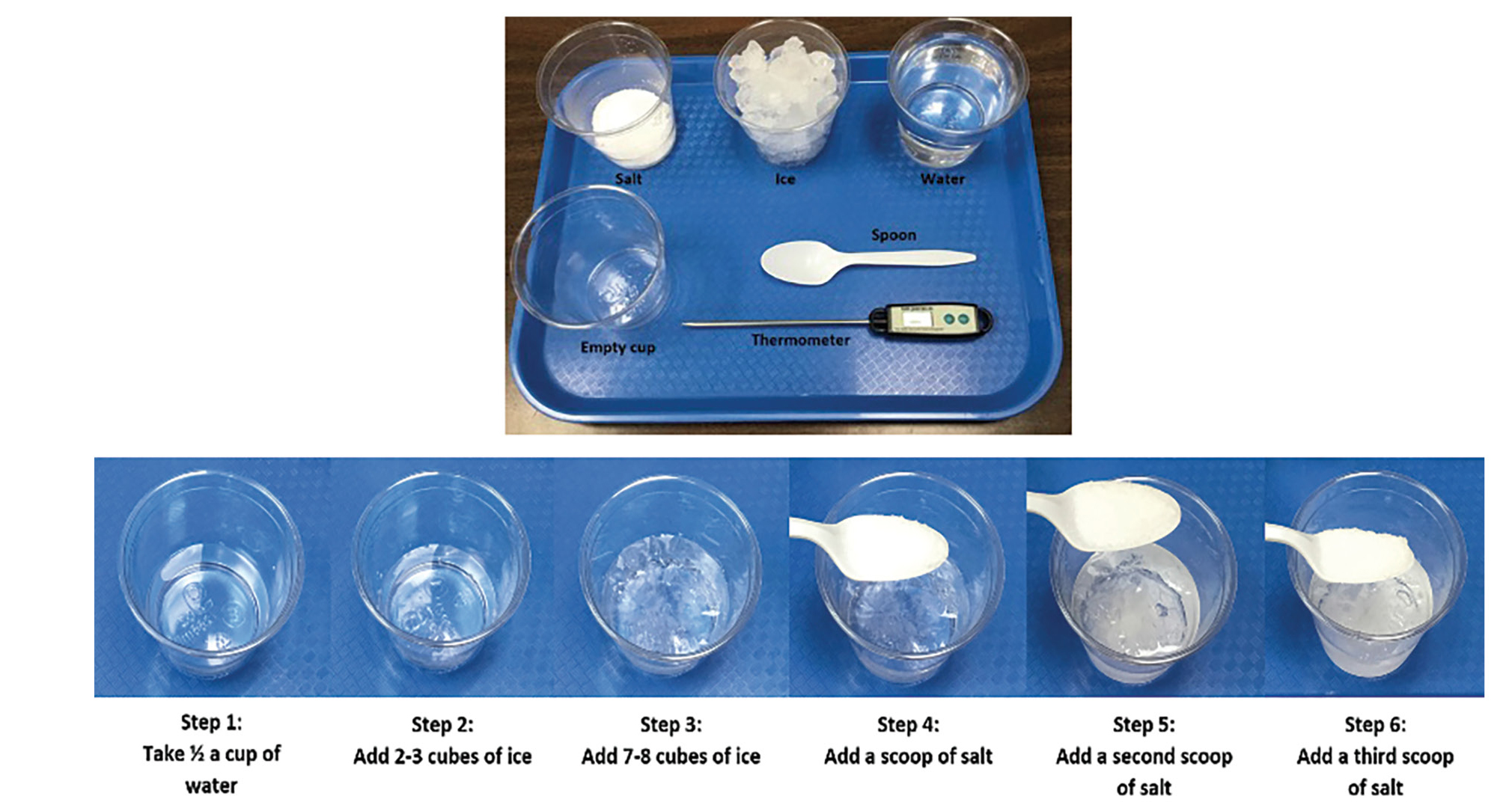
Samples with different combinations of ice and salt to produce different temperatures. The last cup on the right side is a water sample with a digital thermometer.
Discussion Questions
•What do you notice about °F and °C temperatures in various water samples?
•What relationship exists between °F and °C? Explain.
•Why do you think using °C over °F or vice versa would be beneficial?
Before calculating the regression equation, ask students to predict and draw the line of best fit on the graph (Figure 3). Note, the concept of the line of best fit—the line that minimizes the sum of squared differences between the observed and the expected values—will likely need to be discussed as students might be tempted to merely connect individual data points on the graph. This transitional activity of predicting the line of best fit manually helps students strengthen their understanding of the slope-intercept form, which aids them in providing more meaningful interpretations of slope-intercept form in real-world applications Students can also calculate the slope algebraically and find the equation of a line using point-slope form. Discuss that deriving an equation of a line using point-slope form results in students obtaining a slightly different equation to represent the relationship among the same data because each student may choose different sets of data. To overcome this problem, students use the linear regression method, which uses all existing data points. The resulting regression equation will represent the line of best fit and will represent a more accurate relationship between the variables.
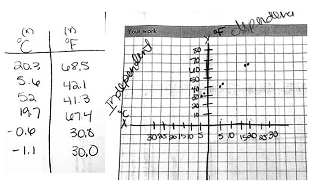
Sample temperature data table and graph generated by the students.
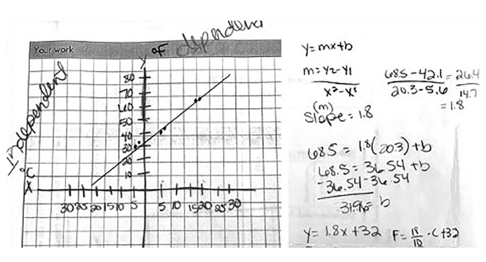
Sample graph and algebraic calculations generated by the students.
Next, students use graphing calculators to find the linear equation using the linear regression method. Students then identify the x and y variables in the graph and substitute in the slope-intercept formula. Students then explain the variables in their equations in a scientific context and compare what they found with the temperature conversion formula.
Step 1: Linear equation y = 1.79x + 31.96
Step 2: Replacing x and y with the variables °F = 1.79°C + 31.96
Step 3: Representing the formula as a fraction °F = 9/5°C + 32
Explain
As a class, students identify the y-intercept and the slope in tabular, graphical, and symbolic representations (Figure 4). Discuss the process of finding the y-intercept and slope from a table, from a graph, or from an equation. Furthermore, discuss the differences and similarities of the representations. Ask students to include the pictorial representation of two thermometers—one in Celsius, one in Fahrenheit—next to the data table to emphasize a real-life connection. Ask probing questions to get students think about the temperature formula and how it was derived. Guide the students to discuss the connections between the mathematical representations and theoretical/physical science concepts. Let the students identify some of the most commonly used formulas in sciences and connect them to the mathematical equations. This discussion should help students see the true integration of math and science.
Elaborate (optional activity)
In this activity students will predict, calculate, and interpret the inverse function of the linear equation from the experiment. Pose a question to students: What happens if the x and y axes of the graph switched? Common answers are that the slope will be negative, the slope will be flipped, and/or the new y-intercept will be –32°C. Allow students to explore by drawing the graph of the inverse function either by hand or by using technology. Once students have their graphs and the equation of the inverse function, they should notice that the y-intercept is –17.7°C (Figure 5).
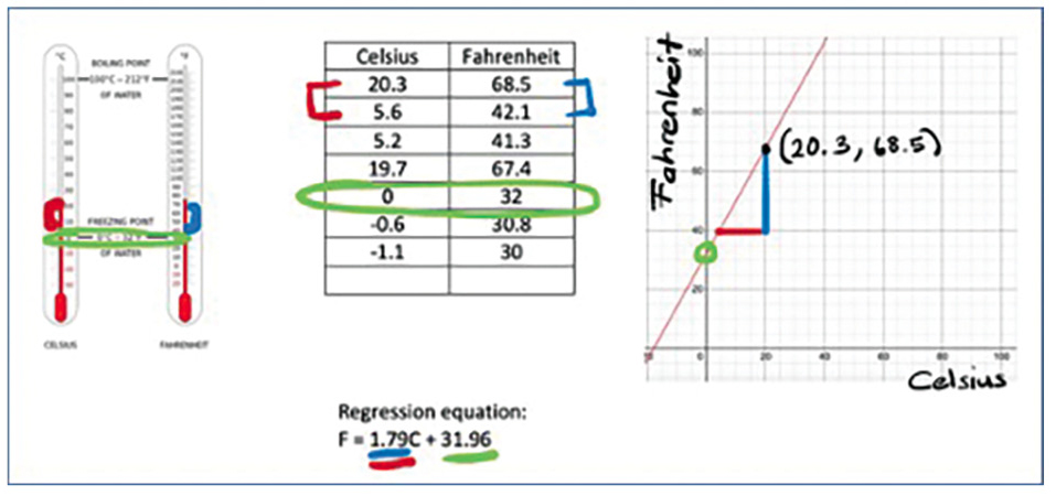
Connecting the information using a visual model, data table, and graph.
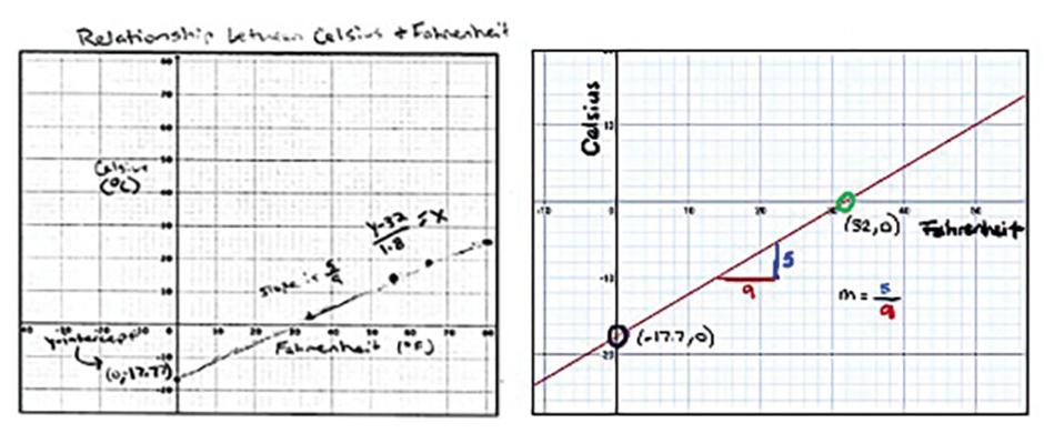
Student work sample showing a graph drawn on paper and a graph generated by using technology.
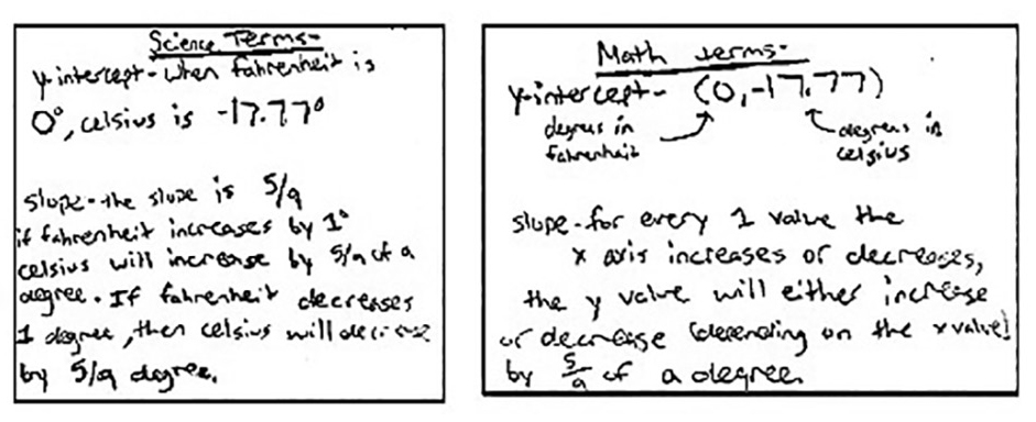
To further clarify students’ misconceptions about the y-intercept, ask students to find the equation of the inverse function algebraically (Figure 6). Students then review the relationship between a function and its inverse. Students may conclude that the x coordinates are switched to y coordinates and y coordinates switched to x coordinates; the y-intercept on the original function would be the x-intercept on the inverse function. They should interpret the slope of the inverse function as a rate of change of °C to °F. Since the variables in the inverse function are switched—the y-axis represents the °C and the x-axis represents the °F—the slope shows the rate change increase in °C for every 1 unit increase in °F (Figure 7).
Evaluate
Finally, the class compares the temperature conversion formula and the linear equation to discuss ways of interpreting the y-intercept and the slope in both scientific and mathematical terms. Sample students’ interpretations of both procedural and conceptual explanation are presented in Table 1. The graph and the interpretations of the y-intercept and the slope in both scientific and mathematical terms can be evaluated using a rubric (see Online Resources, Table 2), a modified version developed by Bright and Joyner (2005).
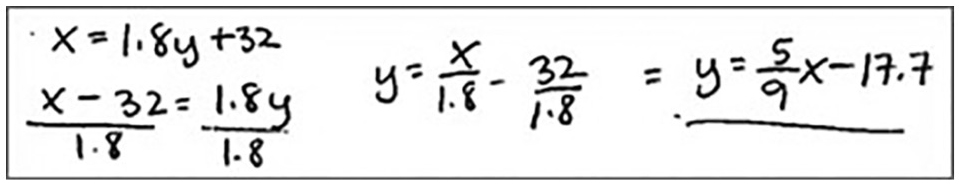
Student work sample showing the equation of the inverse function in an algebraic way.
Student interpretations of the graph.
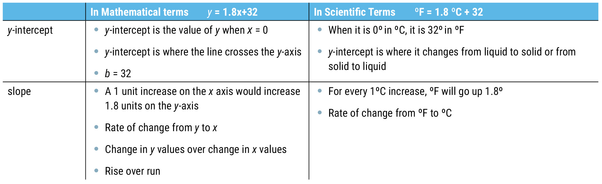
Student interpretations of y-intercept and slope on the linear equation.
Conclusions
Abstract variables used commonly in mathematics, such as x, y, m, and b, take on a concrete meaning when students experience the parallel of those variables while learning scientific concepts. The temperature unit conversion formula provides an interesting context to offer students an opportunity to understand the mathematical concept of linear equation, relate the formula to the slope-intercept form, and apply the mathematical meaning to science principle. Drawing models of Celsius and Fahrenheit thermometers and connecting the labels to parts of the graph and slope-intercept equation provides a visual reinforcement of the concept. Finding alternative-teaching approaches to relate the mathematical representations to commonly used formulas in science give students the opportunity to understand the concepts rather than just memorizing and applying a formula. ■
Online Resources
Table 2 (rubric): https://bit.ly/39EpuxW
Student activity sheet: https://bit.ly/3avcvOr
References
Umadevi Garimella (ugarimel@uca.edu) is the Director at the University of Central Arkansas in Conway, AR. Nesrin Sahin (nesrins@uca.edu) is an assistant professor of mathematics education at the University of Central Arkansas in Conway, AR.
5E Biology Chemistry Crosscutting Concepts Inquiry Interdisciplinary Life Science Mathematics Physical Science STEM High School