
feature
Developing and Using Computer Models to Understand Epidemics

The COVID-19 pandemic is disrupting societies and economies around the world. As of December 2, 2021, COVID-19 had infected more than 264 million people and killed 5.2 million (Center for Systems Science and Engineering [CSSE]). It ranks with the Antonine and Justinian plagues, the Black Death, the depopulation of the Americas, and the 1918 influenza. The pandemic interrupted school and normal life for every student on Earth and is now a fact of daily life.
Infection by the coronavirus SARS-CoV-2 causes COVID-19. An outbreak was first identified in Wuhan, China, in late 2019. By the spring of 2020, the disease had spread across the world and had mutated into many strains. Several strains reached North America by way of Europe and East Asia. Work to identify COVID transmission routes and to control its spread varied by country and region. Many East Asian and Pacific nations reacted to early evidence of respiratory aerosol transmission with effective public health measures. Western public health responses varied, and those of the United States were particularly disorganized and even counterproductive. While public health measures failed in much of the world, medical intervention was a success. Effective vaccines were developed extremely rapidly with new recombinant and RNA-based technologies.
Over the past year, educators have developed curricula teaching about the COVID-19 pandemic (Reed 2020; Royce 2020; Sadler et al. 2020). Many of these curricula feature computer simulations of epidemic dynamics (Kelter 2020; Sadler et al. 2020). Because an epidemic pattern is an emergent property of interacting human behaviors, it is crucial for students to recognize the mechanism of its emergence. Agent-based computer models allow this learning as the computer agents in these models may carry out different behaviors and interactions and organically produce emergent phenomena (Wilensky and Rand 2015).
This article describes an eight-day unit in which students develop their own epidemic simulations and use them to investigate how individual human behaviors and interactions give rise to the epidemic dynamics at the population level (Table 1; see Online Connections). We use NetLogo (Wilensky 1999), a beginner-friendly, agent-based computer modeling tool, to empower students to design and modify their simulations. They collect data, identify patterns, and use mathematical and computational thinking to understand infectious disease spread and control.
Engage (Day 1)
The unit starts with students recalling their experiences related to the COVID-19 pandemic over the past year and sharing their knowledge and questions about COVID-19. After a five-minute class discussion, students consider two questions:
- What is the cause of COVID-19?
- Why is COVID-19 a more severe infectious disease than seasonal flu?
In groups of four, students use a KWL chart (see Day 1 materials) to summarize five facts they know about COVID-19 and three questions they have. They then share with the whole class.
Due to widespread misinformation, many American students may lack prior knowledge of COVID-19 and its severity. For example, they often confuse coronaviruses with bacteria and significantly underestimate how fast COVID-19 may spread.
After students’ misconceptions are identified, students learn about COVID-19 through text and video sources that accommodate students’ reading levels (see Day 1 materials). Students learn that: 1) COVID-19 is caused by the coronavirus, which is much smaller and simpler than bacteria, 2) COVID-19 is transmitted through infectious respiratory aerosols, and 3) coronavirus mainly attacks people’s lungs, but whether people develop severe symptoms depends on their age and health conditions.
Students then study how COVID-19 differs from seasonal flu through relevant reading and videos (see Day 1 materials). A whole-class discussion follows to help students understand that COVID-19 has a different transmission rate, mortality rate, and incubation period than the flu, and therefore may cause severe epidemics, and even a pandemic. Students consider two key questions:
- How do scientists examine an epidemic?
- How do scientists determine whether an intervention may mitigate an epidemic or not?
Some common student misconceptions are that social and news media are reliable sources of information on virus spread and control measures, and that scientists learn about epidemics from the news or social media. The teacher helps students learn that scientists collect real-life data from hospitals, and they may also build computer simulations to study epidemics, predict trends, and test preventive strategies. The day ends with students filling out the “L” section of the KWL chart to explain what they have learned.
Explore (Days 2–4)
On Day 2, students learn about epidemic curves and agent-based computer simulations. Students examine COVID-19 case data from Italy, Germany, and the United Kingdom from February 1–June 30, 2020, and share what they notice and wonder (Figure 1a). Students quickly see that the number of daily new cases first increased and then decreased in all three countries. The teacher prompts students to examine the pattern closely to notice the nonlinear changes, i.e., new cases increasing slowly at first, then more rapidly, and finally dropping at the end. Students then examine new case data from South Korea and Canada for similar patterns (Figure 1b).
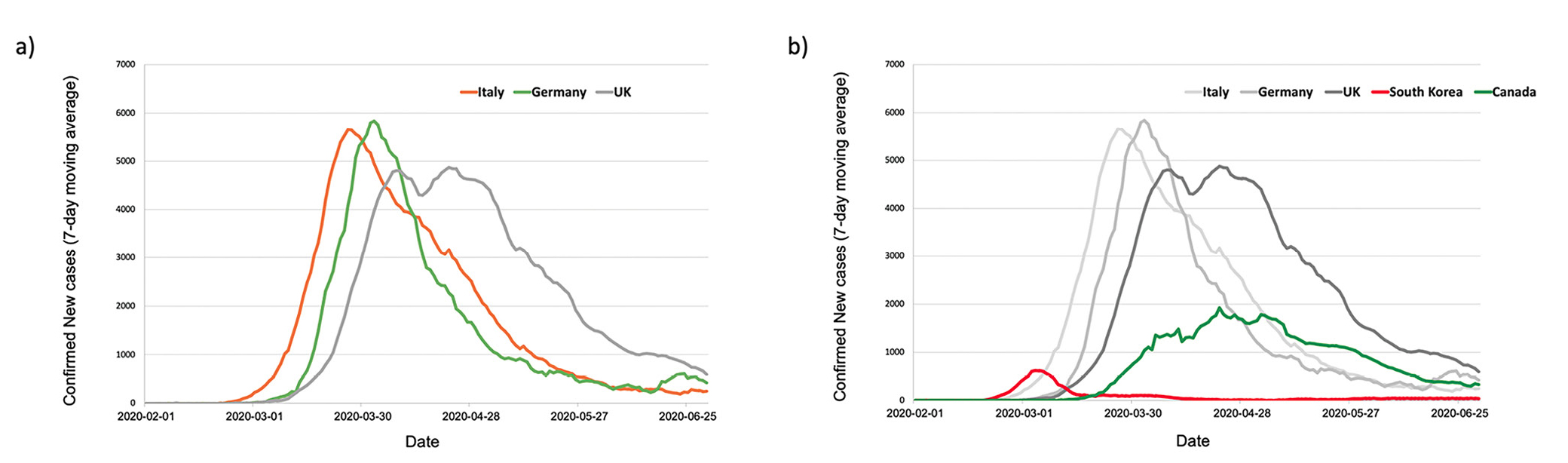
Epidemic curves in five countries from February 1–June 30, 2020.
Students read about this type of trend line, known as an “epidemic curve,” a visual representation of disease progression over an epidemic (see Day 2 materials). Some students wonder if the curve was caused by a different number of people being infected at different times. Some students also notice that trend lines differ among the five countries and wonder why. At this time, the teacher prompts students to consider whether an epidemic computer simulation could help them find the answers. Students investigate agent-based computer models using two videos (see Day 2 materials).
Agent-based computer models (ABM)
An agent-based computer model (ABM) is a type of computer simulation that reveals group behaviors in a system based on the behaviors and interactions of the individual system elements, i.e., agents (Macal 2016). For example, ecologists may simulate population changes in an ecosystem consisting of grass, sheep, and wolves by asking the individual grass patch, sheep, and wolf agents to grow, move, forage, and reproduce. After the agents faithfully enact these behaviors to interact with each other over time, the population fluctuation pattern emerges at the system level (Wilensky and Reisman 2006). NetLogo is a computer modeling tool that allows young students to construct ABMs using a relatively simple programming language (Wilensky 1999). It can be downloaded and installed on PC or Mac platforms for free. Since its development, NetLogo has been used worldwide to study and teach various complex systems.
Students work in pairs or groups of three to explore a bird-flocking simulation in NetLogo for about 10 minutes. They learn that ABMs can simulate flocking by manipulating the individual birds within the group. The flocking behavior is “emergent” because it results from the behaviors of the individual birds. They also learn about the basic features and operations of NetLogo models. Later, students discuss in small groups how bird flocking may relate to infectious disease epidemics and whether the epidemic curve is emergent. This discussion does not aim to fully answer the questions currently but to activate students’ thinking. In the end, students write in their notebooks why or why not they think an epidemic curve is emergent.
On Day 3, students follow a YouTube tutorial (see Day 3 materials) to create a simple ABM simulation. This step takes 25–30 minutes and helps students learn the basic programming routines in NetLogo. Students are excited that they can make a computer simulation and are eager to program more.
Then, students engage in computational thinking (Csizmadia et al. 2015) to plan the epidemic simulation (Table 2; see Online Connections). Under the teacher’s guidance, they dissect an epidemic process by thinking of the stages of COVID-19 people go through: susceptible, exposed, infectious, and recovered (Figure 2). The teacher summarizes the idea using the Susceptible-Exposed-Infectious-Recovered (SEIR) epidemic model (Hethcote 2000) and prompts students to consider:
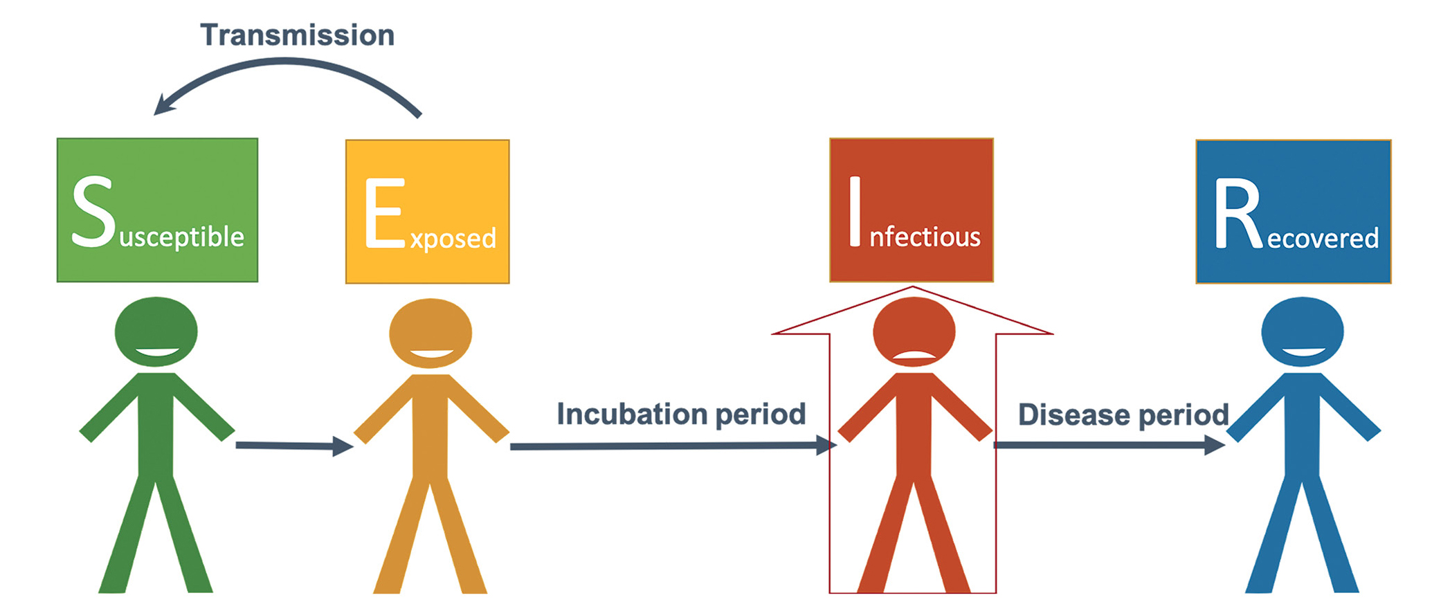
The SEIR epidemic model used in the computer simulation.
- What should be the agents in the epidemic simulation?
- What characteristics should the agents have and not have in a basic epidemic simulation?
- How will the agents behave in the simulation?
- What will happen in the simulation—at first and then what?
In the class discussion that follows, students determine the agents, their properties and behaviors, and come up with a step-by-step scenario in which an exposed carrier comes into a community where all people are susceptible, moves around to contact people, and spreads the disease. These computational thinking discussions conclude Day 3. Students spend all of Day 4 expanding the simple simulation into an epidemic simulation (see Day 4 teaching slides).
Explain (Day 5)
On Day 5 students use the simulation to answer the two questions from Day 2: How does an epidemic curve form? and Why do the COVID-19 epidemic curves vary among different countries? They first compare the real-life epidemic curves with their simulation outputs (Figure 3) and find that the plots of exposed carriers and infectious people show a similar pattern to the epidemic curve. The teacher explains to students that an epidemic curve includes both the carriers and the infectious people in practice. The computer simulation may help us examine the changes in these two infected subgroups closely and separately.
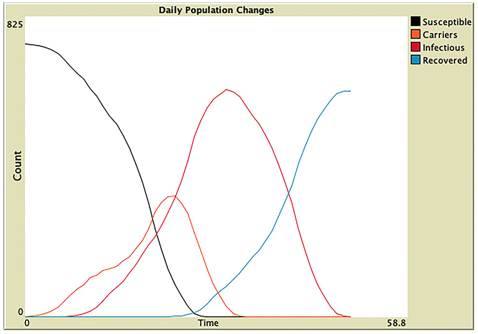
Epidemic simulation outputs.
Students run the simulation tick by tick and quickly notice that the curve pattern emerges from the disease transmission and recovery over time. They share their observation with the class and attribute the curve differences in different countries to the factors they learned from the video on day 1, such as the transmission rate, mortality, or incubation period. The teacher asks students whether and how they may test the ideas in their simulations. Some students propose that they may collect data from the simulation with three such factors varying. The teacher then asks the class to determine how to assess the effects of these factors. Classes often settle on using the maximum daily infectious cases and total deaths as the outcome variables. After the dependent and independent variables are determined, students decide the increment of independent variables and repetitions. Next, the teacher creates a data collection table using a Google spreadsheet and shares it with the whole class. Students collaboratively gather a large data set from the simulation (see Day 5 materials).
The teacher lets students work in small groups to analyze different parts of the data set. Students use mathematical thinking to decide how to represent the data and display the patterns. Figure 4 shows the analyses used to identify the relationships between two factors and the severity of epidemics. In these graphs, students recognize that (1) a higher transmission rate leads to more infectious cases and deaths (Figure 4a and 4b), (2) the number of total deaths is positively associated with both transmission rate and mortality (Figure 4b and 4c), and (3) a longer incubation period leads to more cases and deaths (Figure 4a, 4b, and 4c).
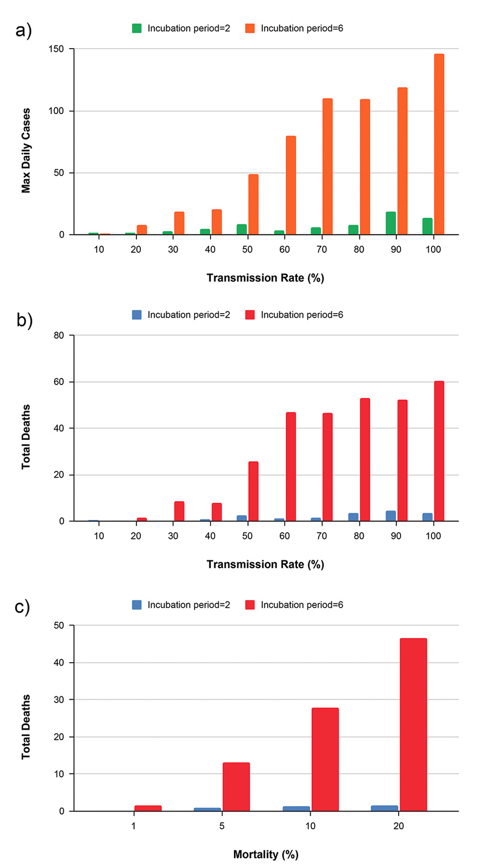
The impacts of the transmission rate, mortality, incubation period on the maximum daily infectious cases (population size = 300).
Next, students work in groups to explain these patterns using the SEIR model and present explanations in class. Students are encouraged to incorporate the agents’ properties and behaviors in their explanations. For example, students may state that because both susceptible and exposed human agents constantly move around in the simulation, and that exposed agents may infect the susceptible, a longer incubation period provides more time for transmission and results in more cases and deaths. Later, students write an evidence-based argument to explain the impacts of two tested factors, e.g., transmission rate and incubation period, on epidemics.
Extend (Days 6–7)
On Day 6, students begin to consider how to control an epidemic. Students brainstorm strategies that may mitigate the COVID-19 epidemic, such as using personal protective equipment (PPE), washing hands frequently and thoroughly, practicing social distancing, and getting vaccinated. Students identify strategies that can be tested in the current simulation. Many realize that using PPE and washing hands can be tested, as these strategies essentially decrease the transmission rates. Still, they need to expand the simulation to test other strategies, such as social distancing and vaccination. From there, the teacher projects the “essential trips only” news photos and asks students why travel restrictions are issued and how they may control COVID-19. Students often propose that travel restrictions may decrease human interactions. Then, students are instructed how to add human mobility as a variable in the epidemic simulation to investigate its impact.
It should take students less than five minutes to update their simulations (see teaching slides) and about 10 minutes to collaboratively collect data. Based on the new data, students find that increasing mobility in the simulation elevates both maximum daily cases and total deaths (Figure 5). In the simulation, students can directly observe how lower levels of mobility decrease interactions among people, therefore reducing disease spread. Students are excited the simulation supports their reasoning.
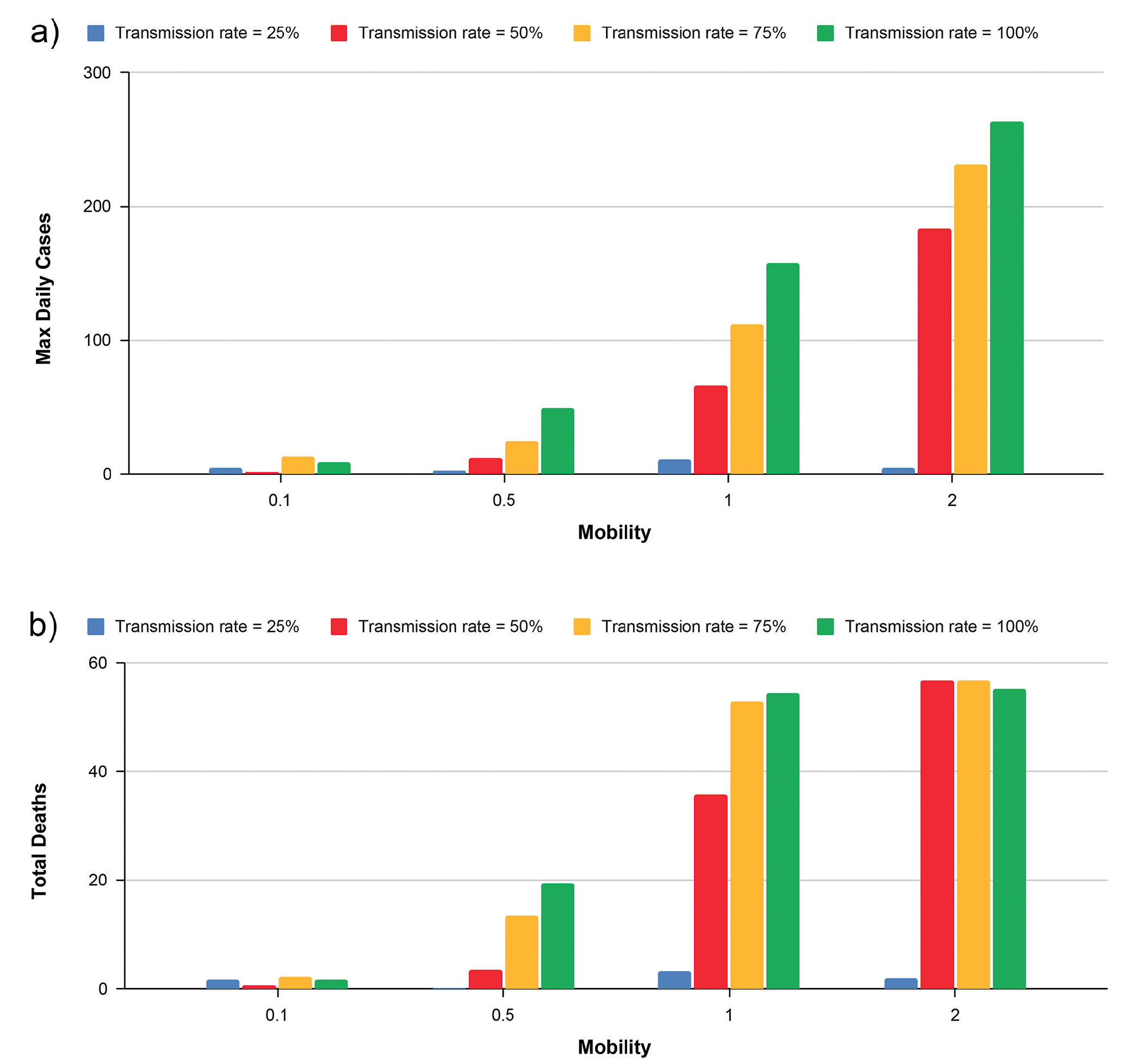
The impacts of mobility levels on the maximum daily cases and total deaths (population size = 300).
At this time, students compare the infectious curves from the mobility levels of 1 and 0.5 in a less dense population, holding other factors constant. Students can see the curve is flatter when mobility is lower (Figure 6a and 6b). Using these graphs from the simulation, students understand the idea of “flattening the curve” (Figure 6b) and recognize that flattening the infectious curve decreases the number of daily cases and avoids overwhelming the public healthcare system.
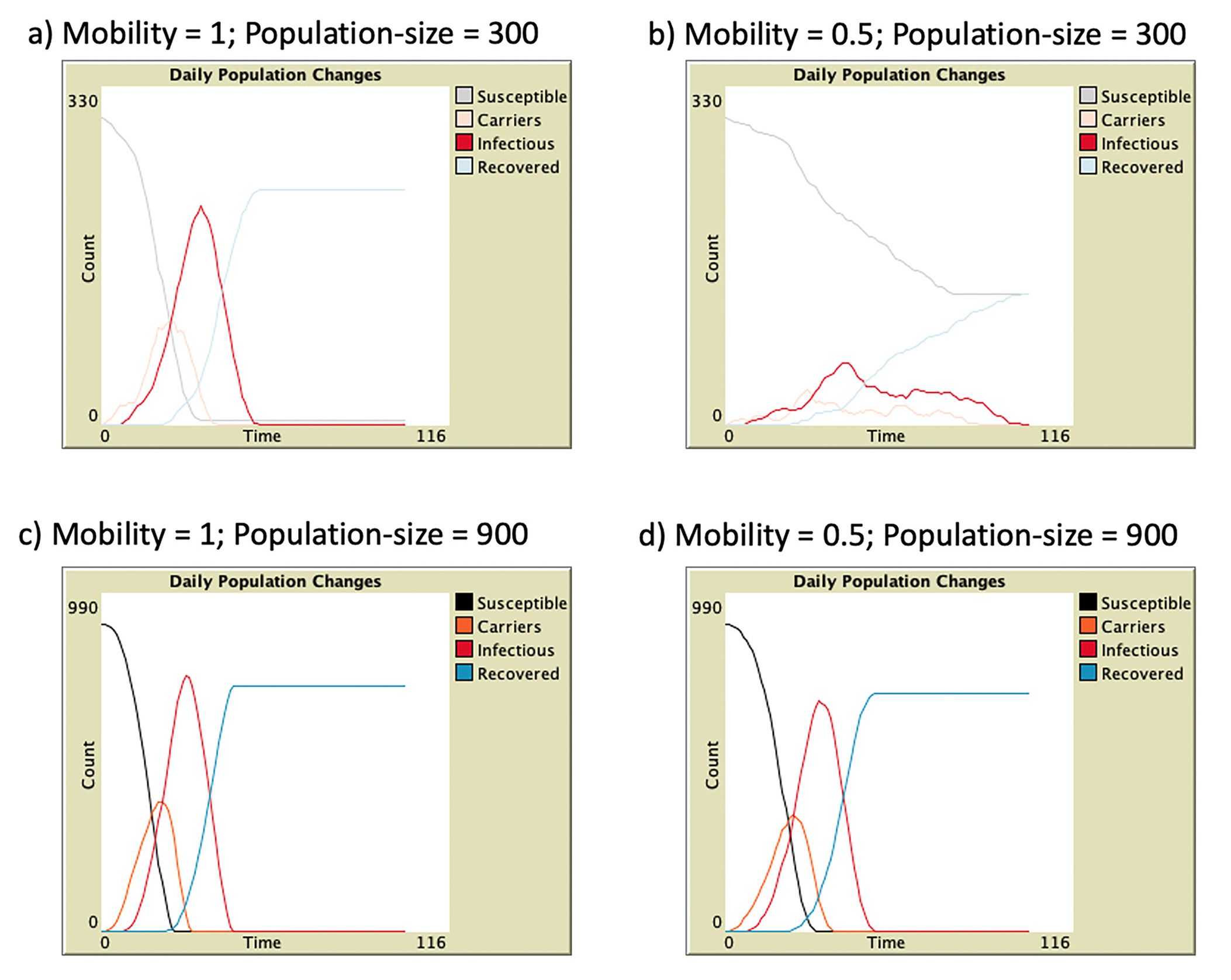
Computer simulation shows the levels of mobility influence the infectious curve more effectively in a less dense population than in a dense one.
The teacher prompts students to consider if the same result occurs in a denser population. Students use the simulation to find that the levels of mobility have small impacts on a dense population (Figure 6c and 6d). Students may relate the results to real-life situations, such as crowded factories and school classrooms. Here, the teacher points out that practicing social distancing is a more effective strategy in those situations. Students examine a ready-made simulation of social distancing (see Day 6 materials) to compare the effect of social distancing with that of population mobility. In the end, students construct a written argument to explain how and when travel restrictions may mitigate epidemics.
On Day 7, the teacher presents a COVID-19 curve graph spanning from February 2020–January 2021 (Figure 7). These graphs show that the existing control strategies have not yet contained COVID-19 by January 2021 and raise the question: What else can we do to control COVID-19 effectively? Some students may propose the vaccination as a solution. The teacher lets students share some questions they have about vaccination. The most asked questions include what a vaccine is, how it differs from an antibiotic, how it works, and what side effects vaccines have. Then, students watch two videos to learn about vaccination and herd immunity (see Day 7 materials). They are challenged to think about:
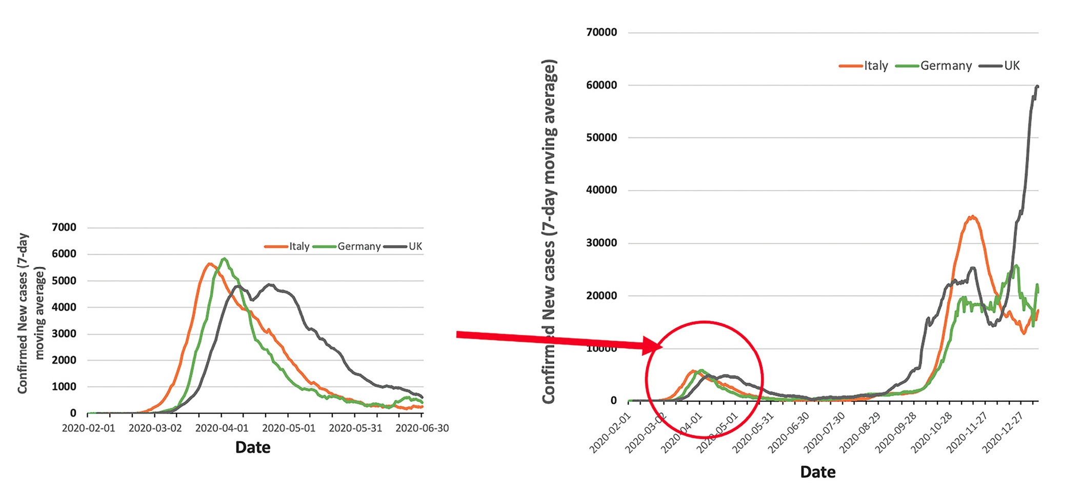
The COVID-19 data graphs revealing the pandemic continues.
- What percentage of a population should be vaccinated to achieve herd immunity?
- What factors affect the herd immunity threshold?
At this point, some students ask how they can test the effect of vaccination and answer the questions using the simulation. The teacher holds a class discussion on the properties and behaviors of vaccinated agents in the simulation, and then shows students how to add the vaccination component into the epidemic simulation. Students take about 25–30 minutes to expand the simulation, collaboratively gather data, and analyze the data.
Based on the results, students conclude that a higher herd immunity threshold is needed for more transmissible diseases or in a more crowded population (Figure 8). Then students read two articles about herd immunity and vaccinations related to COVID-19 to further their understanding (see Day 7 materials). The day ends with students writing an argument about the impact of vaccination rates on the COVID-19 pandemic supported by evidence from the computer simulation.
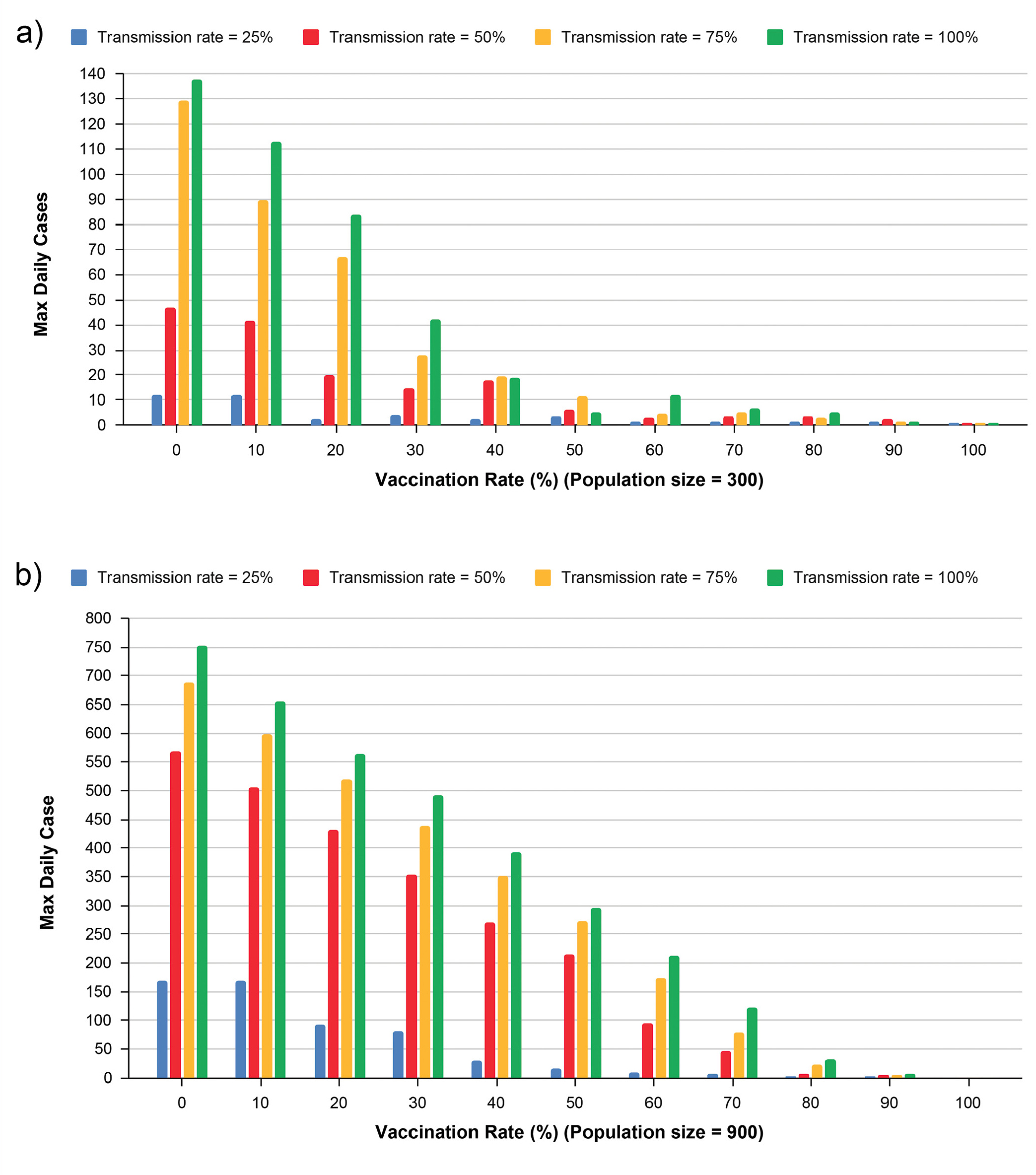
The effects of vaccination rates on maximum daily cases in a population of 300 (a) and a population of 900 (b).
Evaluate (Day 8)
Students have developed, used, and revised agent-based computer models to investigate the spread and control of infectious diseases over the previous seven days. On Day 8, students reflect on the modeling process. It is important for students to recognize both the merits and limitations of computer simulations. Comic reading is provided to broaden students’ views on the complexity of modeling epidemics (see Day 8 materials). The class discusses how they can simulate a complex real-world problem like an infectious disease epidemic by breaking down the system into small components and a set of behavioral rules.
Computer simulations provide a visual and dynamic representation of a complex system that is hard to study using traditional methods. A computer simulation may reveal the internal interactions of a system, predict system behaviors, and test solutions. Students also realize that computer simulations only capture certain aspects of the system. Scientists must use real-world data to develop and validate computer simulations. The incorporation of real-world information may improve the explanatory and predictive power of a computer simulation.
Students are encouraged to consider how they could improve their simulation. Some student ideas include differentiating agents’ age and mortality, adding superspreaders, differentiating transmission rates for agents wearing and not wearing PPE, and including asymptomatic but contagious people.
Finally, students write a one-page letter to the public explaining why controlling the COVID-19 pandemic depends on everyone doing their part. Students are prompted to include the SEIR model, data from the simulation and empirical observation, and epidemic prevention strategies in the letter. The letter is shared in the class to receive peer comments and feedback.
Conclusion
In this agent-based modeling unit, students investigate infectious disease spread and control. The focus on the current COVID-19 epidemic should be engaging for high school students. The curriculum empowers students to develop their own computer simulations and conduct mathematical thinking to study a real-world phenomenon. We have field-tested this curriculum with several groups of high school students and teachers, many of whom had no experience with NetLogo or with programming. Table 3 (see Online Connections) outlines scaffolding strategies with which teachers may differentiate their teaching. Students with all levels of programming experience will gain experience with computational modeling, and will be empowered to use contemporary computational tools to explore and understand complex processes such as the COVID-19 pandemic. ■
Online Connections
Lin Xiang (lin.xiang@uky.edu) is an assistant professor of science education in the Department of STEM Education at the University of Kentucky, Lexington, KY; Scott Diamond (scott.diamond@fayette.kyschools.us) is a high school science teacher at Fayette County Public Schools, Lexington, KY.
5E Instructional Materials Life Science STEM Three-Dimensional Learning High School