
feature
Surface-X
Modeling Scanning Tunneling Microscopy (STM) in the classroom
Teaching the tools and concepts associated with modern physics can often be a daunting and difficult task for secondary science teachers. Classical physics is often perceived as intimidating and complex in its own right. Modern physics addressing quantum phenomena where Newtonian laws break down is even more abstract for learners. However, comprehending these concepts is critical to understanding modern technology and scientific instruments (Angell et al. 2004).
One such instrument is the scanning tunneling microscope. Scanning tunneling microscopy (STM) is a method used to image surfaces at the atomic level. It involves moving an extremely fine, electrically charged needle across a sample surface in a vacuum chamber. The needle is made of tungsten and is only one atom in size at its tip. As the needle scans over the surface in near contact with it, electrons will jump, or tunnel, across the gap between its tip and the atoms below (University of Texas at Dallas 2018).
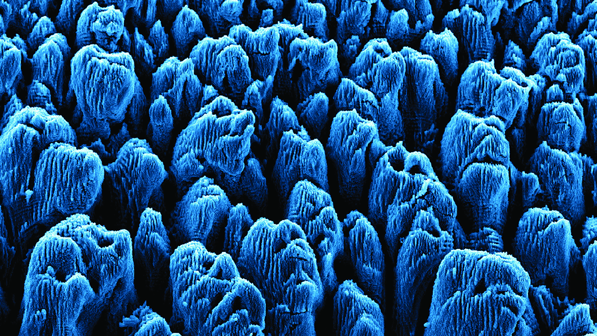
Scientists can either measure the change in current flowing between the needle and the atoms on the surface, or they can measure the changes in topography of a surface by maintaining a constant current level and moving the needle accordingly. Based upon the size and electron properties of each atom, a different current will be measured. These differences in current can then be turned into an image to show the individual atoms composing a given surface (Rohrer 1990). The following image from Chiang (2011) shows a three-dimensional rendering of an image captured using STM.
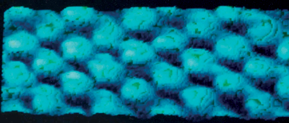
Three-dimensional rendering of an image captured using STM
Along with imaging, STM allows scientists to rearrange and change the properties of individual atoms, which has tremendous implications for understanding surfaces and their applications in nanotechnology or data storage (Rohrer 1990). One scientist using this instrument is Ellen D. Williams, professor of physics at the University of Maryland. Her work involves the use of STM to study surface characteristics in next-generation electronic materials such as graphene and organic semiconductors for applications in nanotech. She hopes to combine technology and biological models to build quantum computers and error-correction capability in next-generation technological systems. Such work could result in improved technology available for all people, while lowering the environmental and ecological footprint associated with modern electronics (Ahmed 2008).
In order to simulate STM, the process had to be brought up to a much larger scale and integrate technologies that students were already familiar with. The learning objectives associated with this activity emphasize understanding the concepts of STM imagery, practicing science and engineering process skills, using data collection and analysis to build a model, and integrating technology to collect data and generate a 3-D computer model. The activity described in this article is intended to take two to three class periods (approximately three hours of instructional time) and uses materials and equipment that are inexpensive and readily available on any school campus. Additionally, students have a hand in building their own probes and composing their own surfaces, further cementing cross curricular concepts learned in other classes or disciplines. Students are also given the opportunity to create a three-dimensional rendering of a surface, giving them transferable experience in data entry and analysis. Our process can be modified to include student participation at various points in preparing the materials. It can also be easily differentiated to address different concepts or ability levels.
Activity Components and Assembly
The following materials (costs included as applicable) were used to create the Surface-X activity: Copy paper boxes Standard sized (8.5” × 11”) cardstock (approximately 16 sheets) Tape (masking or electrical) Scissors Craft glue Materials of various conductivity (aluminum foil, conductive paper (available through Pasco for $67 for 100 sheets), charcoal pencils, different grades of artist pencils) Plastic balloon sticks ($12.99 for 100 sticks) Thin gauge (16-20) enameled copper wire (magnet wire) ($17 per 320ft) Sand paper Button battery ($22 per 100 pack) LEDs ($10 per 200) Digital multimeter ($12 per unit)
Step 1: Building the Box
We built the box simulating the STM vacuum chamber using a printer paper box. Such boxes are usually found for free in abundance in copy rooms on school campuses. They are ideal because they have lids that are easily removable and are already sized to fit two sheets of standard paper. To create the chamber, cut the box in half to reduce its height to approximately 10 to 15 cm. A grid of 5 mm diameter holes placed two or three cm apart can then be punched in the top using a large nail or pencil tip. This is the most time-consuming part of the materials preparation for the activity and should be done outside of instructional time. Boxes can be numbered in order to keep track of which lab groups or students have which box with which surface. Using a lab tech or teacher’s aid is recommended. The finished product should look like the box shown in Figure 1.
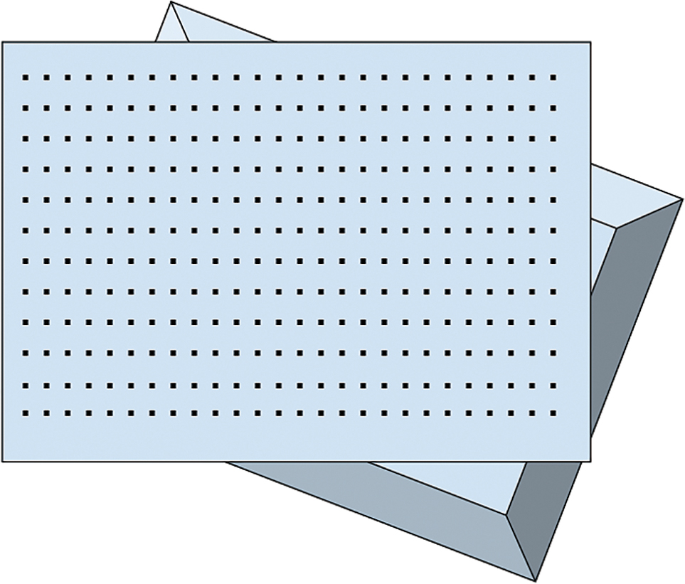
Sample box with hole pattern
If an instructor wishes to make a more permanent box, then flat plastic storage containers with lids can be substituted. These can be bought as a pack of 8 measuring 13. 6in. × 18. 5in. × 5. 49in for $48 through online retailers. Holes can be drilled in the lid and the inside can be spray painted or lined with paper as necessary to conceal the contents of the box. One added advantage of using plastic storage containers is their ability to be stacked to minimize space during storage. If using a plastic box, building the surface on a large sheet of cardboard or foam core is recommended.
Step 2: Creating the Surfaces
In order to measure the current for an unknown surface, the materials used to create the surface should be conductive. If the image is to be more intricate or complicated, materials of largely different conductivity should be used. Materials such as aluminum foil, conductive paper, charcoal pencils, and different grades of graphite art pencils (6H to 6B) have different levels of conductivity and are very effective at creating a varied surface topography.
To create the surface substrate, two pieces of standard size (8.5” × 11”) cardstock can be taped together on the long side to make a single surface that is 17” × 11” in area. Surface components can then be glued onto the substrate sheet in various designs based on real crystalline structures or imaginary forms. Surfaces can be assembled with any number of shapes or configurations based on the appropriate instructional level and content. The surface designs that have been used in this activity have been modeled after actual metallic or crystalline surfaces.
The different materials can be used to represent atoms of different elements. Figure 2 shows an example of a surface that can be achieved using materials of different conductivity in different configurations to replicate a known crystalline surface. Creating the surfaces can be time-consuming and should be done outside of instructional time using a teacher’s aide or lab tech if available. Once complete, place the surface in the box and cover with a lid to conceal the contents.
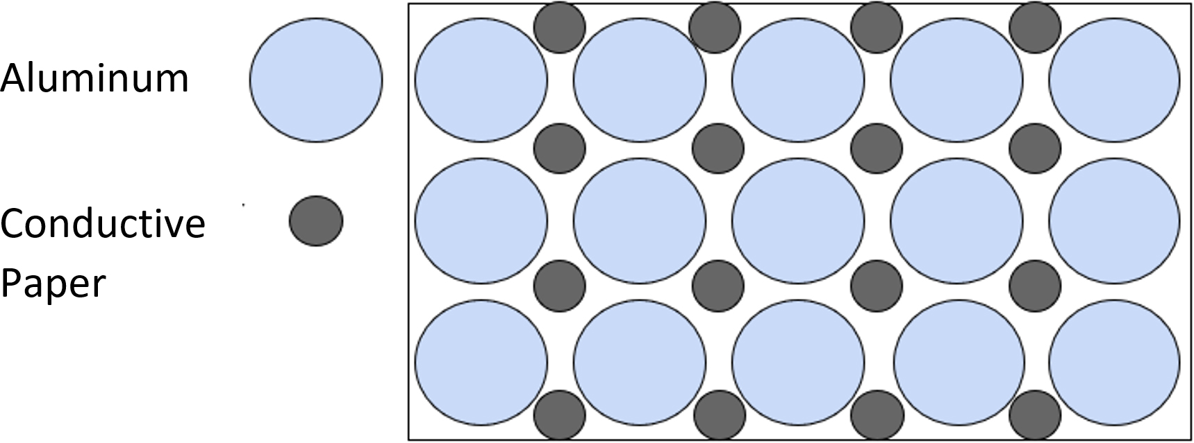
Example conductive surface pattern.
Step 3: Creating the Probe
There are two options for creating a probe to measure the conductivity of the point of the surface being measured. The first involves using the qualitative brightness of a LED classified in categories of very bright, medium bright, dim, very dim, or no light at all. A very conductive material would result in a very bright light. A material with low conductance, such as a graphite pencil, would result in a dim or very dim light.
The second (and more expensive) option uses a digital multimeter to gather quantitative data in the form of current through the sampled regions of the simulated surface. It helps to have a sample card with the different materials on it so that students can observe the differences in brightness and compare to what they observe when taking measurements from the box.
The probes are easy to construct and test, requiring no more than 15-20 minutes of instructional time. Parts for the probes can be gathered into separate bags or envelopes for easy distribution. Students can work with a partner to build their probes in order to reduce the amount of material required.
To build the probe, follow the steps below: 1.Start by cutting one plastic balloon stick in half. Plastic balloon sticks are ideal because they are cheap, rigid, durable, and hollow like a straw. 2.Cut two pieces of insulated copper wire so that they are approximately five centimeters longer than the section of balloon stick. Using a small piece of sandpaper, remove about one centimeter of insulation from both ends of each wire. 3.Thread the wire through the balloon stick so that one sanded end of each wire is just past the end of the balloon stick. Fold the sanded end of each wire back over the edge of the balloon stick and secure with a layer of electrical tape. The two bent ends at the end of the balloon stick should be bare wire and will be used to complete the circuit when in contact with a conductive surface 4.Two long pieces of wire should be sticking out of the top end of the balloon stick. Tape one sanded end of one wire to the negative side of a button battery. 5.Taking one LED, tape the positive (longer) leg of the LED to the positive side of the button battery. 6.Tape the negative (shorter) leg of the LED to the sanded end of the remaining copper wire.
The simple probe is now complete. Test it out on various conductive surfaces such as aluminum foil (very bright), conductive paper (bright), or even moistened skin (very dim) to make sure it works. Figure 3 shows the first option probe design using the qualitative LED brightness as a measure of surface conductivity.
Illustration of a completed LED option probe.
To create a probe that will use a digital multimeter with alligator clips to measure current as quantitative data, construct the probe as described above. However, instead of attaching a LED to the positive side of the battery, tape one end of a third short piece of wire approximately five centimeters in length and sanded on both ends to the positive side of the battery.
Using alligator clips attach the two free ends of wire to the leads of a digital multimeter. Figure 4 shows the second option quantitative probe design using a digital multimeter.
Illustration of a completed DMM option probe.
Collecting Data
The data collection portion of the activity may take 30–45 minutes to complete. To collect data, students (working on tables or stations in groups of two to four) will need to have a numbered box with an unknown sample, a probe, and a sheet of graph paper. It is best to have boxes at the front of the room and only allow students to obtain them once they have a working probe. Students should create a grid of dots on their graph paper that mimics the holes in the top of their box.
Students should then start scanning their sample, taking readings by inserting their probe into every hole in the top of the box. The probe tip should come into gentle contact with the surface on the bottom of the box but should not be jammed or forced. Working with their partner, one student should probe the box while the other writes the observed measurement on the gridded graph paper. Up to four students can work at the same time on a single box. Depending on the type of probe used students should write either the current in milliamps from the display on the digital multimeter or they should write the brightness of the LED as a scale of zero to four according to the list below beside each lid hole’s corresponding location on their data grid.
- Very Bright =4
- Bright = 3
- Dim = 2
- Very Dim = 1
- No Light = 0
Analysis: Creating a Two-Dimensional Image
Students should spend any time left in class to begin creating images of their surfaces; they can also complete this portion of the activity as homework outside of instructional time. Once students have gathered their data they should begin trying to draw contour lines in order to create closed shapes around regions that have generally the same value range. They should then color in the shapes they created using a different color pencil for each enclosed value range. The progression should look like the images shown in Figure 5.
Example pattern progression for a 2D surface representation.
Creating a Three-Dimensional Image
To further integrate technology and build computer modeling skills, students can use Microsoft Excel—available in classroom computers, computer labs, or home computers to create a three-dimensional image of the surface they measured. To accomplish this, students should Open a New Sheet in the program. Leaving the first cell (A1) blank, they should place a numbered sequence starting at the number one across the first row and down the first column to represent the number of rows and columns of holes they had in the lid of their box. They should then fill in the grid they created with the numerical data from their graph paper as shown in Figure 6.
Sample data grid
After entering their data, they should highlight their entire table, select “insert” from the toolbar, select “recommended charts”, then select “all charts”, then select “surface”. The program will generate a three-dimensional rendering of the surface based on the data in the table they created. Students can rotate the graph to observe the surface model from different angles. Overhead and perspective views of the three-dimensional graph for data grid in figure 6 are shown below in figure 7.
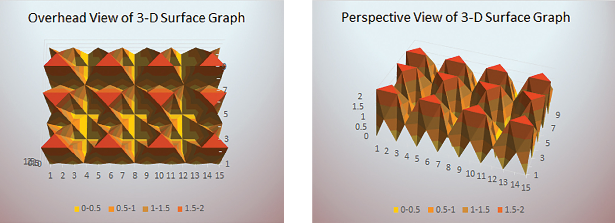
Overhead and perspective view examples of a 3D representation.
A Black Box Conclusion
Black box is an exercise described by Latour (2003) as a means of drawing conclusions about an unseen object that is enclosed in a box based upon empirical evidence that can be gathered by manipulating the box. Whatever is in the box remains unseen, even at the conclusion of the exercise. The use of the black box examination technique has gained ground as an exercise in empirical investigations across upper and lower grade levels (Chakrabarti, Pathare, Huli, and Nachane 2013) (Rode and Friege 2017) in the design concepts of modern science centers and museums (Toon, 2005).
In keeping with the spirit of modeling STM, the students never get to look in the box. They may only make inferences and draw conclusions based on the data they collect. Just as scientists who use STM cannot directly observe the surface they are looking at, students must rely only on data they gather using technology.
However, students can still discuss sources of error or inaccuracies. They can discuss how they can modify their boxes, surface characteristics, or probes in order to increase the accuracy and precision (resolution) of their final rendering.
Students can be assessed based on their use of laboratory instructional time, the quality of their surface renderings, the accuracy of their surface renderings (how close their rendering matches the surface in the box), and their ability to answer conclusion or extension questions identifying sources of error, discussing ways to improve accuracy and precision, and how STM might be used to improve modern technology. A simple rubric may be designed to assess the following criteria: Quality of data collected in the form of grid values on a table (Figure 6) Quality of final images produced (two-dimensional, three-dimensional, or both) (Figures 5 and 7) Accuracy of the rendered surface compared to what was actually in the box (known only to the teacher) Quality of answers to conclusion or analysis questions.
This activity can be modified to address multiple STEM topics, particularly any application that relies on probes or remote data such as ground-penetrating radar, underwater sonar, weather balloons, or even radio telescopes. For instance, a teacher could make various templates of landscapes, fossils, or geological features (submerged island chain, subduction zone (trench), rift zones, wrecks, etc.) located on the ocean floor. Students could use their probes to simulate sonar in order to create an image of that feature. Students could then identify each feature based on the image they render. To connect the learners culturally they could create a surface rendering of a physical place or a chemical surface that exists in their country or state of origin.
To differentiate the activity for gifted learners, the rigor could be increased by providing students with the parts for a probe and having them design and fabricate one themselves using only prior knowledge. They could also have surfaces that mimic actual substances such as silicon, copper, or sodium, and then they would have to identify their surfaces accurately based on the rendering they produce and images of known chemical structures or crystal lattices. Accelerated learners could also conduct independent research about the uses and applications of STM and propose a way to apply the technology to their own fields of interest.
To differentiate this activity for challenged learners, students could create a picture of their own design out of conductive materials and place them in the box. Other students can then probe the box attempting to recreate the design in their rendered images as an exploration of resolution and digital imagery technology. Challenged learners could also work in groups, use a box lid with fewer holes, or use a very simplified surface to reduce the amount of data collection required while still maintaining the concept and requirements of the activity. Teachers could also provide challenged learners with pre-drawn templates of the surface (similar to step 2 in Figure 5) and have students color them using a prescribed key based on their observed data in a paint-by-number format.
Conclusion
Much of modern science and technology involves using a probe of some sort to gather data about a surface that is not directly observable or accessible. The utilization of probes to explore properties of a surface or a phenomenon involves engineering, data gathering, and analytical skills in order to arrive at a new understanding. However, integrated science processes are not adequately incorporated in the classroom and tend to give way to basic science skills, especially moving from primary to secondary education (Yamusak 2016).
Furthermore, understanding process skills improves students’ attitudes toward and willingness to learn scientific subject matter (Kamba 2018). The integration of science process skills also helps to bridge the achievement gap in non-traditional and disenfranchised learners (Montgomery and Wray 2018).
Lastly, Kramer and Walston (2019) found that using integrated science process skills in science instruction improved students’ understanding of the interdisciplinary nature of science. Much as Ellen D. Williams moved from chemistry to modern physics, students who may have been exclusively interested in only one field of science may now be more willing to explore other science disciplines, improving their science knowledge and abilities on the whole.
The activity described in this article integrates many science process skills and is an excellent addition to STEM studies. It not only directly simulates scanning tunneling microscopy, but it also can be extended to address multiple disciplines and scientific processes. This activity helps students not only conceptualize an instrument that relies on quantum phenomena, but also improves students’ science process skills, improves their attitude toward learning a difficult concept, and encourages them to relate this field of study to other scientific fields of interest to them.
Acknowledgment
The author would like to thank the physics department at University of California Riverside for their expert feedback related to the development of this activity.
Danny McKinney (drdannymckinney@gmail.com) is a STEM/Science Instructor at North County High School in Glen Burnie, MD.
5E Careers Crosscutting Concepts Engineering Instructional Materials Labs Lesson Plans NGSS Physical Science Physics Science and Engineering Practices STEM Teacher Preparation Teaching Strategies Technology Three-Dimensional Learning High School Grades 9-12